学习论文 Zero-shot Learning via Simultaneous Generating and Learning笔记_综合

Notation

$θ\theta$ :represents the parameters of the deep neural network that define the decoder.
$ψ\psi$ :represents the parameters of the deep neural network that define the encoder.
$q?(z∣x,y)q_{\phi}(z|x,y)$ :traditional encoder,作为目标识别模型，need y for both training and testing

如果对概率图模型的随机变量的向量 $X$ , $Z$ 进行建模得到的生成模型 $pθ(x)=∑zpθ(z)pθ(x∣z).p_{\theta}(x)=\sum_zp_{\theta}(z)p_{\theta}(x|z).$ 一般此求和式不可以写成有限运算形式，故无法通过ML算法优化，同时第二项的似然 $pθ(z∣x)=pθ(x,z)pθ(z)p_{\theta}(z|x)=\frac{p_{\theta}(x,z)}{p_{\theta}(z)}$ 中含有的prior也不可计算（p(z)是隐变量的概率，这是我要采样转化的，但是目前seen很少，无法得到转化的概率分布，不然还求啥p(x)）
所以用AEVB算法， $q?(z∣x,y)q_{\phi}(z|x,y)$ 近似似然 $p_{theta}(z|x)$ 同时把最大化似然函数下界作为目标函数的方法，巧妙地避开了后验概率计算。（听不懂没关系，禁止套娃记结论）

$pθ(x∣z,y)p_{\theta}(x|z,y)$ :traditional decoder, 是隐变量的后验分布，need y for both training and testing

Cause $y$ , when labels missing, both encoder and decoder are hardly
exploited and decoder only takes advantage when generating datapoints
in certain condition

If adopting assume: $p(z∣y)→p(z)p(z|y)\rightarrow p(z)$ ,exploiting the latent variables for classification becomes new challenge.

$A^*$ :class attribute embedding vectors
$p(Xs?∣Ays?)p(X^{s*}|A^{s*}_y)$ 将类别用类嵌入向量 $A ?$ 表示，通过中间隐变量 $z$ 生成 $x$ 的过程
$pψ(z∣a)p_{\psi}(z|a)$ :attribute-specific gaussian distribution of z.

$μ(xs?)\mu(x^{s*})$ :the mean of the approximated variational likelihood $q?(z∣xs?)q_{\phi}(z|x^{s*})$
$p(x∣ayu?)?∫zpθ^(x∣z)pψ^(z∣ayu?)p(x|a^{u*}_y)\simeq \int_z{p_{\hat{\theta} } (x|z)p_{\hat{\psi} }(z|a^{u*}_y) }$ :GENERATIVE MODEL,generate unseen sampled datapoints for [18]
$Θ^\hat{\Theta}$ :generative model parameters need optimized.
$x^I$ 辅助变量

Abbreviation

SGAL: Simultaneously Generating And Learning

Motivation

1.Problem

Traditional models are trained mainly on the seen classes. Obtaining the generative model for
both seen and unseen is quite far from their consideration, since scarcity of the unseen samples is apparently a fundamental problem for ZSL.

2.Existing Solution and Difficulty

CVAE: generate conditional samples
GAN
Difficulty: Need training additional off-the-shell classifier

Those methods based on deep generative model train their models first and generate enough samples for unseen classes and subsequently train additional classifier, rather than training conditional generative models for both seen and unseen classes.

Contribution of this paper

数据问题：为了推理大量含有missing label $y$ 的数据，无中生有，逼近其真实的标签，传统VAE面临unknown intent identify的问题，Assuming that categories represented as class embedding vectors $a^*$ ,模型学习attribute-specific的潜在空间分布，再通过隐变量生成 $x$ （曲线救国）
任务驱动：since our purpose is classification（not just generative）,assuming the conditional prior to be a category-specific Gaussian distribution ，所以引入最大化间隔准则来促使 $q?(z∣xs?)q_{\phi}(z|x^{s*})$ 与其他类别的 $pψ(z∣ays??)p_{\psi}(z|a^*_{y^{s*}})$ 越远越好.(Trick: Margin Regularizer)
训练过程：treat these missing datapoints as variables that should be optimized as well as
model parameters. 把这些missing的数据点对应分布的参数当做变量（EM参数估计），作为整个模型参数优化的一部分，随生成模型训练参数优化更新而一并更新（个人感觉是这篇文章的重点工作）

Methodology

给出了class semantic(or attribute) embedding vectors $A?={ak?}k=1S+UA*=\{a^*_k\}^{S+U}_{k=1}$ including both seen and unseen的属性向量，为attribute-specific方法做准备。

1 Category-Specific Multi-Modal Prior and Classification

Input variable independently: the latent prior $p(z∣y)→p(z)p(z|y)\rightarrow p(z)$ , and exploiting the latent var $z$ for classification
VAE可以通过隐变量学习数据的复杂模型。不同于标准VAE的隐变量z的先验分布是服从标准正态分布，我们假设每个zn是从attribute-specific的高斯分布 $pψ(z∣ays??)p_{\psi}(z|a^*_{y^{s*}})$ 得到的

Inductive ZSL

Standard VAE prior: 隐变量 $z_n$ 从高斯分布 $pψ(zn)=N(0,I)p_{\psi}(z_n)=N(0,I)$ 采样得到。
attribute-specific VAE prior:隐变量的先验从高斯分布 $pψ(zn∣an)=N(μ(an),∑(an))p_{\psi}(z_n|a_n)=N(\mu (a_n),\sum (a_n))$ 采样得到。

根据Inductive ZSL method,考虑seen class $X^{s*}$ 和对应的类别向量标签 $Ays?A^{s*}_y$ 的概率关系已知用边界似然。目的是建立隐变量 $z$ 与seen数据的属性向量之间的映射关系，从而解决了大量missing label $y$ 情况下无法通过现有real $x$ 生成 $z$ 的问题。其VAE下边界变成： $L(Θ;xs?,ayis??)=?KL(q?(z∣xs?∣∣pψ(z∣ayis??))+Ez?q[logpθ(xs?∣z)]L(\Theta;x^{s*},a^*_{y^{s*}_i})=-KL(q_{\phi}(z|x^{s*}||p_{\psi}(z|a^*_{y^{s*}_i}))+E_{z\sim q}[log p_{\theta}(x^{s*}|z)]$
既然目标是先生成 $z$ ，那么就需要建立 $z$ 与 $ayis??a^*_{y^{s*}_i}$ 的映射。继续Assuming that条件先验概率 $pψ(z∣ayis??)p_{\psi}(z|a^*_{y^{s*}_i})$ 是category-specific Gaussian distribution的，那么 $ayis??a^*_{y^{s*}_i}$ 就是一个样本空间的可数无限的划分，满足全概率公式 $P(A)=∑nP(A∣Bn)P(Bn)P(A)=\sum_nP(A|B_n)P(B_n)$ ，因此就可以计算隐变量的概率分布： $p(z)=∑ip(ayis??)pψ(z∣ayis??)p(z)=\sum_ip(a^*_{y^{s*}_i})p_{\psi}(z|a^*_{y^{s*}_i})$
得到 $z$ 的先验目的是为了分类，而如何能够让不同先验值的 $z$ 更加简单清晰地反映不同类别呢？
作者采用属性向量归一化和先验正则化Loss的方法promotes each cluster of $pψ(z∣ayis??)p_{\psi}(z|a^*_{y^{s*}_i})$ to be far away from all other clusters above the certain distance in latent space $z$
再通过KL散度 $(q?(z∣xs?∣∣pψ(z∣ayis??))(q_{\phi}(z|x^{s*}||p_{\psi}(z|a^*_{y^{s*}_i}))$ 得到的encoder $q?(z∣xs?)q_{\phi}(z|x^{s*})$ 就可以逼近不可解的条件似然 $pψ(z∣ayis??)p_{\psi}(z|a^*_{y^{s*}_i})$ ，这是VAE的经典之处，即经典的intractability 问题

intractability:
$pθ=∫pθ(z)pθ(x∣z)dzp_{\theta}=\int p_{\theta}(z)p_{\theta}(x|z)dz$ ,公式不可以写成有限运算的形式，则不可计算，故无法通过ML算法进行参数优化。同时 $pθ(z∣x)=pθ(z,x)/pθ(x)p_{\theta}(z|x)= p_{\theta}(z,x)/p_{\theta}(x)$ 中含有先验概率也不可计算，故无法使用EM算法对参数进行优化以及进行所有基于后验概率的推理。为了解决这个问题，VAE采用 $q?(z∣x)q_{\phi}(z|x)$ 近似 $pθ(z∣x)p_{\theta}(z|x)$ 同时把最大化似然函数下界作为目标函数的方法，巧妙地避开了后验概率计算。这一过程数学工具与模型与上文一致。

最后回到优化问题上，利用MLE方法对label $y^\hat y$ 估计： $y^=argmaxys?p(xs?∣ayis??)?argmaxys?pψ(z=μ(xs?)∣ays??)\hat y=argmax_{y^{s*}}p(x^{s*}|a^*_{y^{s*}_i})\simeq argmax_{y^{s*}} p_{\psi}(z=\mu (x^{s*})|a^*_{y^{s*}})$
其中 $μ(xs?)\mu (x^{s*})$ 就是上式边界的先验似然逼近函数 $q?(z∣xs?)q_{\phi}(z|x^{s*})$ 的均值。

By simply calculating Euclidian distances between category-specific multi-modal and the encoded variable $μ(xs?)\mu (x^{s*})$ ,classification results can be achieved.（不同类别转化成不同参数的高斯分布，通过分布的均值区别不同的类别（你用方差也行））

We train the model using the seen-class labeled examples and learn the parameters $Θ^\hat {\Theta}$ by maximizing the objective in $L(Θ;xs?,ayis??)L(\Theta;x^{s*},a^*_{y^{s*}_i})$ .Once the model parameters have been learned, the label for a new input $x^\hat x$ from an unseen class can be predicted by first predicting its latent embedding $z^\hat z$ using the VAE recognition model, and then finding the “best” label by solving $y^=argmaxyu?L(Θ,x^,Ayu?)=argmaxyu?p(x^∣ayiu??)?argmaxyu?pψ(z=μ(xu?)∣ayu??)\hat y=argmax_{y^u*}L(\Theta,\hat x,A^{u*}_y)=argmax_{y^{u*}}p(\hat x|a^*_{y^{u*}_i})\simeq argmax_{y^{u*}} p_{\psi}(z=\mu (x^{u*})|a^*_{y^{u*}})$
就可以生成unseen的 $x^\hat x$ 的 $y^\hat y$ （ the model is trained on seen classes $A^{s?}$ , we can try to use the generative model by simply inputting the embedding vector of unseen classes $^{u?}$ ）

2 Generative Model for both Seen and Unseen Classes

Focus: training process, the absence of datapoints Xu? for unseen classes is a fundamental problem
in ZSL.
So treat these missing datapoints as variables that should be optimized as well as model parameters.
反向思维，假设lower bound已经完美的逼近了我们的target distribution for both seen and unseen class，边界参数 $Θ\Theta$ 和unseen datapoint $X^{u*}$ 会同时满足：

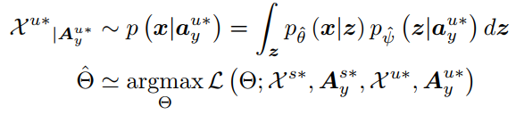
这是生成模型常见的一种递归学习方法。从生成器
$pθ^(x∣z)pψ^(z∣ayu?)p_{\hat \theta}(x|z)p_{\hat \psi}(z|a^{u*}_y)$ 采样得到missing datapoint $X^{u*}$ ，在用这个采样的batch和seen existing datapoints $X^{s*}$ 一起喂回去优化生成器参数 $Θ^=argmaxΘ∑k=1S1N∑xn?p(x∣aks?)Nlogp(xn∣aks?;Θ)\hat \Theta=argmax_{\Theta}\sum^S_{k=1}\frac{1}{N}\sum^N_{x_n\sim p(x|a^{s*}_k)}logp(x_n|a^{s*}_k;\Theta)$ 。并通过SGAL递归求解上面两式完成模型参数训练。但是注意啊，我们采的missing datapoint 不是瞎采样的，而是需要采样的 $X^{u*}$ 近似服从我们的unseen classes $p(x|a^{u*})$ 这样一个target likelihood.
但是我们并不知道target likelihood是什么…（如果我们是有监督学习，我们就知道目标分布是什么样子，但是现在unseen烦就烦在不知道这货的分布是什么）

所以这里需要EM算法，既然我不知道精确分布，我估计一个大致分布也可以啊。

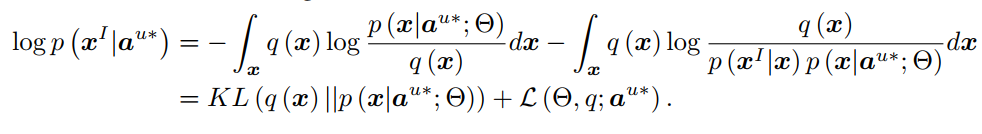
其中 $x$ 和 $x^I$ are assumed to be a feature vector and its corresponding image,We assume that generating $x$ is only affected by $a$ , and $x^I$ is depend only on $x$ .

使用EM算法的目的，就是要把这货分布的参数 $Θ\Theta$ 给估计出来,那就对对数似然函数求导嘛：

对比一下 $Θ^=argmaxΘ∑k=1S1N∑xn?p(x∣aks?)Nlogp(xn∣aks?;Θ)\hat \Theta=argmax_{\Theta}\sum^S_{k=1}\frac{1}{N}\sum^N_{x_n\sim p(x|a^{s*}_k)}logp(x_n|a^{s*}_k;\Theta)$ 和 $argmaxΘ∑k=S+1S+U1N∑xn?p(x∣aku?;Θold)Nlogp(xn∣aku?;Θ)argmax_{\Theta}\sum_{k=S+1}^{S+U}\frac{1}{N}\sum_{x_n\sim p(x|a^{u*}_k;\Theta^{old})}^Nlogp(x_n|a^{u*}_k;\Theta)$

采用EM算法的参数优化方法，与传统方法的区别在：

previous model采样 $xn?p(x∣aku?;Θold){x_n\sim p(x|a^{u*}_k;\Theta^{old})}$ 过程，将unseen的属性向量作为了先验知识（与上文unseen + existing labeled datapoint对应），作为算法的E-step；
VAE方法逼近真实分布的参数 $Θ\Theta$ ,作为算法的M-step: $L(Θ;xs?,ayis??)=?KL(q?(z∣xs?∣∣pψ(z∣ayis??))+Ez?q[logpθ(xs?∣z)]L(\Theta;x^{s*},a^*_{y^{s*}_i})=-KL(q_{\phi}(z|x^{s*}||p_{\psi}(z|a^*_{y^{s*}_i}))+E_{z\sim q}[log p_{\theta}(x^{s*}|z)]$

算法的structure，感觉其实还不如直接看算法流程

但是在EM算法迭代优化 $Θ\Theta$ 的过程中，由于存在 $X^u$ is generated from the incomplete model which is still in the training process(不确定性问题), thus handle the uncertainty by assuming the model parameters to be Bayesian random variables. (也就是说对生成器模型 $pθ^(x∣z)pψ^(z∣ayu?)p_{\hat \theta}(x|z)p_{\hat \psi}(z|a^{u*}_y)$ 进行处理）

生成器中的unseen classes $pψ^(z∣ayu?)p_{\hat \psi}(z|a^{u*}_y)$ 可以展开为：

The model uncertainty can be considered by activating dropouts in each network.

3 More Conclusion of the structure

2.13号又继续看了一下作者的代码部分，感觉前面对文章中prior network理解的不够彻底，没有提及这一关键的structure,正如作者的注释：

#==================== VAE structure example =========================
# vaeStructure = {
    
# 'name' : 'VAE',
# 'encoder': {
    
# 'name' : 'encoder',
# 'trainable' : True,
# 'inputDim' : 2048,
# 'hiddenOutputDimList' : [512, 128],
# 'outputDim' : 128*2,
# 'hiddenActivation' : tf.nn.leaky_relu,
# 'lastLayerActivation' : None,
# },
#
# 'decoder': {
    
# 'name' : 'decoder',
# 'trainable' : True,
# 'inputDim' : 128,
# 'hiddenOutputDimList' : [512],
# 'outputDim' : 2048,
# 'hiddenActivation' : tf.nn.leaky_relu,
# 'lastLayerActivation' : None,
# },
#
# 'priorNet': {
    
# 'name' : 'priorNet',
# 'trainable' : True,
# 'inputDim' : 85,
# 'hiddenLayerNum' : 2,
# 'outputDim' : 128,
# 'hiddenActivation' : tf.nn.leaky_relu,
# 'lastLayerActivation' : None,
# 'constLogVar' : None,
# },
# }

priorNet是针对采样sampling部分的一个先验网络，在上文中的EM部分的M step( Step 2)对应着 $E?E_{\phi}$ ，为什么采用先验网络也是为了方便cluster的一个操作，具体可以参考参考文献32，讲得十分详细。
Encoder和Decoder部分的代码基本和传统VAE理解思路是一样的。

Appendix

Margin Regularizer

The objective in $L$ naturally encourages the inferred variational distribution $q?(z∣x)q_{\phi}(z|x)$ to be close to the class-specific latent space distribution $pθ(z∣x)p_{\theta}(z|x)$ . However, since our goal is classification, we augment this objective with a maximum-margin criterion that promotes $q?(z∣x)q_{\phi}(z|x)$ to be as far away as possible from all other class-specific latent space distributions.