原文链接:https://www.kaggle.com/gzuidhof/full-preprocessing-tutorial/notebook
Introduction
Working with these files can be a challenge, especially given their heterogeneous nature. Some preprocessing is required before they are ready for consumption by your CNN.
Fortunately, I participated in the LUNA16 competition as part of a university course on computer aided diagnosis, so I have some experience working with these files. At this moment we top the leaderboard there :)
This tutorial aims to provide a comprehensive overview of useful steps to take before the data hits your ConvNet/other ML method.
What we will cover:
- Loading the DICOM files, and adding missing metadata
- Converting the pixel values to Hounsfield Units (HU), and what tissue these unit values correspond to
- Resampling to an isomorphic resolution to remove variance in scanner resolution.
- 3D plotting, visualization is very useful to see what we are doing.
- Lung segmentation
- Normalization that makes sense.
- Zero centering the scans.
Before we start, let's import some packages and determine the available patients.
英文不咋好,只能意译,没有办法一字不漏的翻译。见谅。如有错误,请大家指正。
介绍
处理这些文件是一种挑战,特别是考虑到他们成分的复杂性。在将他们送进CNN网络之前,一些预处理是必不可少的。
幸运的是,我曾经参加过LNUA16比赛,所以我对处理这些文件有点经验。
这个教程目的在于提供有用的步骤的概览,以便于将这些数据应用与你们的网络。
主要内容:
- 加载DICOM文件,添加缺失的metadata
- 将像素值转换为亨氏单位(肺部组织对应的单位)
- 重采样到同构(同样)分辨率,以消除扫描分辨率的差异。
- 3D绘点(绘图),可视化能让我们明白究竟在做什么。
- 肺部(图片)切割。
- 归一化。
- 零中心化。
Before we start, let's import some packages and determine the available patients.
%matplotlib inlineimport numpy as np # linear algebra
import pandas as pd # data processing, CSV file I/O (e.g. pd.read_csv)
import dicom
import os
import scipy.ndimage
import matplotlib.pyplot as pltfrom skimage import measure, morphology
from mpl_toolkits.mplot3d.art3d import Poly3DCollection# Some constants
INPUT_FOLDER = '../input/sample_images/'
patients = os.listdir(INPUT_FOLDER)
patients.sort()
Loading the files
Dicom is the de-facto file standard in medical imaging. This is my first time working with it, but it seems to be fairly straight-forward. These files contain a lot of metadata (such as the pixel size, so how long one pixel is in every dimension in the real world).
This pixel size/coarseness of the scan differs from scan to scan (e.g. the distance between slices may differ), which can hurt performance of CNN approaches. We can deal with this by isomorphic resampling, which we will do later.
Below is code to load a scan, which consists of multiple slices, which we simply save in a Python list. Every folder in the dataset is one scan (so one patient). One metadata field is missing, the pixel size in the Z direction, which is the slice thickness. Fortunately we can infer this, and we add this to the metadata.
加载文件
DICOM是医疗图像的文件标准。这是我第一次处理DICOM,但事实上处理起来还是相当顺利的。这些文件包含很多metadata(中文翻译:元数据)(例如像素尺寸,所以在现实世界中在每个维度中一个像素有多长呢)。
这些每个扫描文件的像素尺寸各不相同,会影响CNN的表现。后面我们会使用同构重采样解决这个问题。
下面的代码是加载一份扫描文件。扫描文件包含多个切片,我们将其简单地存储在python列表中。数据集中的每个文件夹
都是一份扫描文件(对应一名病人)。缺少一个元数据字段,即Z方向 的像素大小,即片厚。幸运的是我们能推断这一点,并将其添加到元数据中。
# Load the scans in given folder path
def load_scan(path):slices = [dicom.read_file(path + '/' + s) for s in os.listdir(path)]slices.sort(key = lambda x: float(x.ImagePositionPatient[2]))try:slice_thickness = np.abs(slices[0].ImagePositionPatient[2] - slices[1].ImagePositionPatient[2])except:slice_thickness = np.abs(slices[0].SliceLocation - slices[1].SliceLocation)for s in slices:s.SliceThickness = slice_thicknessreturn slices
The unit of measurement in CT scans is the Hounsfield Unit (HU), which is a measure of radiodensity. CT scanners are carefully calibrated to accurately measure this. From Wikipedia:
By default however, the returned values are not in this unit. Let's fix this.
Some scanners have cylindrical scanning bounds, but the output image is square. The pixels that fall outside of these bounds get the fixed value -2000. The first step is setting these values to 0, which currently corresponds to air. Next, let's go back to HU units, by multiplying with the rescale slope and adding the intercept (which are conveniently stored in the metadata of the scans!).
在CT的扫描测量的单位是Housfield单位(亨氏),这是一个衡量放射密度的单位。CT扫描仪经过仔细校准以精确测量。从维基百科:
(见上表)
但是,默认情况下返回的值不在这个单位中。让我们来解决这个问题。
有些扫描仪有柱面扫描边界,但输出图像是正方形的。在这些边界之外的像素得到固定值-2000。第一步是将这些值设为0,该值当前对应于空气。接下来,让我们回到亨氏单位,乘以(rescale)重新调节的斜率再加上截距(方便存储在扫描文件的元数据中)。
def get_pixels_hu(slices):image = np.stack([s.pixel_array for s in slices])# Convert to int16 (from sometimes int16), # should be possible as values should always be low enough (<32k)image = image.astype(np.int16)# Set outside-of-scan pixels to 0# The intercept is usually -1024, so air is approximately 0image[image == -2000] = 0# Convert to Hounsfield units (HU)for slice_number in range(len(slices)):intercept = slices[slice_number].RescaleInterceptslope = slices[slice_number].RescaleSlopeif slope != 1:image[slice_number] = slope * image[slice_number].astype(np.float64)image[slice_number] = image[slice_number].astype(np.int16)image[slice_number] += np.int16(intercept)return np.array(image, dtype=np.int16)first_patient = load_scan(INPUT_FOLDER + patients[0])
first_patient_pixels = get_pixels_hu(first_patient)
plt.hist(first_patient_pixels.flatten(), bins=80, color='c')
plt.xlabel("Hounsfield Units (HU)")
plt.ylabel("Frequency")
plt.show()# Show some slice in the middle
plt.imshow(first_patient_pixels[80], cmap=plt.cm.gray)
plt.show()Resampling
A scan may have a pixel spacing of [2.5, 0.5, 0.5], which means that the distance between slices is 2.5millimeters. For a different scan this may be [1.5, 0.725, 0.725], this can be problematic for automatic analysis (e.g. using ConvNets)!
A common method of dealing with this is resampling the full dataset to a certain isotropic resolution. If we choose to resample everything to 1mm1mm1mm pixels we can use 3D convnets without worrying about learning zoom/slice thickness invariance.
Whilst this may seem like a very simple step, it has quite some edge cases due to rounding. Also, it takes quite a while.
Below code worked well for us (and deals with the edge cases):
重采样
扫描文件可以具有[2.5,0.5,0.5]的像素间距,这意味着片与片之间的距离为2.5毫米。一个不同的扫描文件的像素间距可能是[1.5,0.725,0.725],这在自动分析(使用卷积神经网络)上是有问题的。
一个普遍的处理这个问题的方案是,对整个数据集重采样成一定的各向同性分辨率。如果我们选择将每一个扫描文件重采样为[1,1,1]像素间距,就无需顾虑不同的切片厚度使用3D卷积神经网络。
虽然这似乎是一个非常简单的步骤,但它由于四舍五入有相当多的边缘情况。并且,这需要很长的时间。
def resample(image, scan, new_spacing=[1,1,1]):# Determine current pixel spacingspacing = np.array([scan[0].SliceThickness] + scan[0].PixelSpacing, dtype=np.float32)resize_factor = spacing / new_spacingnew_real_shape = image.shape * resize_factornew_shape = np.round(new_real_shape)real_resize_factor = new_shape / image.shapenew_spacing = spacing / real_resize_factorimage = scipy.ndimage.interpolation.zoom(image, real_resize_factor, mode='nearest')return image, new_spacingPlease note that when you apply this, to save the new spacing! Due to rounding this may be slightly off from the desired spacing (above script picks the best possible spacing with rounding).
Let's resample our patient's pixels to an isomorphic resolution of 1 by 1 by 1 mm.
请注意,在执行上面的函数时,要保存新的间距。由于四舍五入,这可能会导致轻微偏离所需要的间距(以上的脚本选择最好的四舍五入间距(其实这里不是很明白啊))。pix_resampled, spacing = resample(first_patient_pixels, first_patient, [1,1,1])
print("Shape before resampling\t", first_patient_pixels.shape)
print("Shape after resampling\t", pix_resampled.shape)Shape before resampling (134, 512, 512)
Shape after resampling (335, 306, 306)3D plotting the scan
For visualization it is useful to be able to show a 3D image of the scan. Unfortunately, the packages available in this Kaggle docker image is very limited in this sense, so we will use marching cubes to create an approximate mesh for our 3D object, and plot this with matplotlib. Quite slow and ugly, but the best we can do.
绘制3D扫描图def plot_3d(image, threshold=-300):# Position the scan upright, # so the head of the patient would be at the top facing the camerap = image.transpose(2,1,0)verts, faces = measure.marching_cubes(p, threshold)fig = plt.figure(figsize=(10, 10))ax = fig.add_subplot(111, projection='3d')# Fancy indexing: `verts[faces]` to generate a collection of trianglesmesh = Poly3DCollection(verts[faces], alpha=0.70)face_color = [0.45, 0.45, 0.75]mesh.set_facecolor(face_color)ax.add_collection3d(mesh)ax.set_xlim(0, p.shape[0])ax.set_ylim(0, p.shape[1])ax.set_zlim(0, p.shape[2])plt.show()Our plot function takes a threshold argument which we can use to plot certain structures, such as all tissue or only the bones. 400 is a good threshold for showing the bones only (see Hounsfield unit table above). Let's do this!
plot_3d(pix_resampled, 400)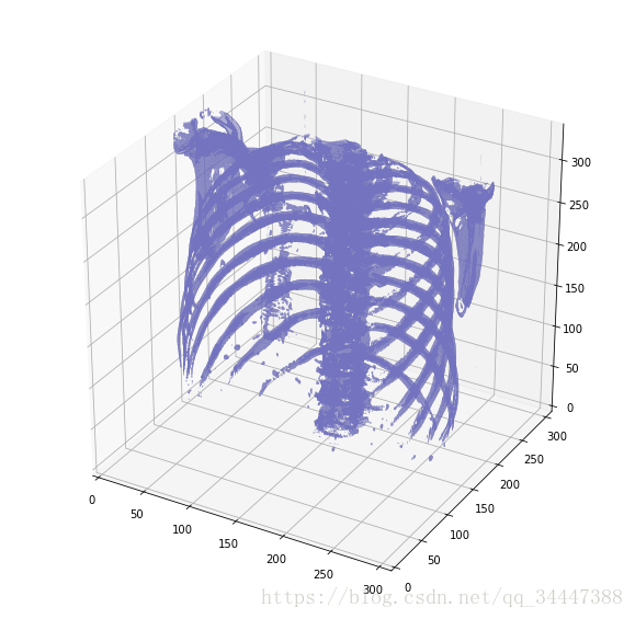
哇,瘆人!
Ps.
运行上述代码可能会出现问题,plot_3d里面改一下: marching_cubes-》marching_cubes_classic
Lung segmentation
In order to reduce the problem space, we can segment the lungs (and usually some tissue around it). The method that me and my student colleagues developed was quite effective.
It involves quite a few smart steps. It consists of a series of applications of region growing and morphological operations. In this case, we will use only connected component analysis.
The steps:
- Threshold the image (-320 HU is a good threshold, but it doesn't matter much for this approach)
- Do connected components, determine label of air around person, fill this with 1s in the binary image
- Optionally: For every axial slice in the scan, determine the largest solid connected component (the body+air around the person), and set others to 0. This fills the structures in the lungs in the mask.
- Keep only the largest air pocket (the human body has other pockets of air here and there).
这涉及到几个不少巧妙的步骤。它包括区域生长和形态学运算的一系列应用。在这种情况下,我们只使用连接(有关联的)组件分析。
步骤为:
- 给图像设定阈值(-320HU是一个很好的阈值,但这并不重要)
- 做连接组件(不是非常懂),确定周围空气的标签,在二进制图像中填充1.
- 可选:对扫描文件中的每个轴向切片,确定最大的固体连接组件,设置其他为0.这填补了肺部结构的mask。
- 只保留最大的气囊(人体内还有其他的气囊)。
def largest_label_volume(im, bg=-1):vals, counts = np.unique(im, return_counts=True)counts = counts[vals != bg]vals = vals[vals != bg]if len(counts) > 0:return vals[np.argmax(counts)]else:return Nonedef segment_lung_mask(image, fill_lung_structures=True):# not actually binary, but 1 and 2. # 0 is treated as background, which we do not wantbinary_image = np.array(image > -320, dtype=np.int8)+1labels = measure.label(binary_image)# Pick the pixel in the very corner to determine which label is air.# Improvement: Pick multiple background labels from around the patient# More resistant to "trays" on which the patient lays cutting the air # around the person in halfbackground_label = labels[0,0,0]#Fill the air around the personbinary_image[background_label == labels] = 2# Method of filling the lung structures (that is superior to something like # morphological closing)if fill_lung_structures:# For every slice we determine the largest solid structurefor i, axial_slice in enumerate(binary_image):axial_slice = axial_slice - 1labeling = measure.label(axial_slice)l_max = largest_label_volume(labeling, bg=0)if l_max is not None: #This slice contains some lungbinary_image[i][labeling != l_max] = 1binary_image -= 1 #Make the image actual binarybinary_image = 1-binary_image # Invert it, lungs are now 1# Remove other air pockets insided bodylabels = measure.label(binary_image, background=0)l_max = largest_label_volume(labels, bg=0)if l_max is not None: # There are air pocketsbinary_image[labels != l_max] = 0return binary_imagesegmented_lungs = segment_lung_mask(pix_resampled, False)
segmented_lungs_fill = segment_lung_mask(pix_resampled, True)plot_3d(segmented_lungs, 0)
Beautiful!
But there's one thing we can fix, it is probably a good idea to include structures within the lung (as the nodules are solid), we do not only want to air in the lungs.
漂亮!plot_3d(segmented_lungs_fill, 0)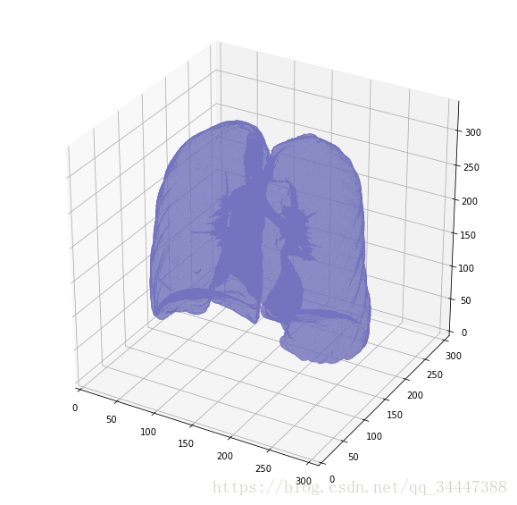
更好了。让我们来看看他们俩的区别。
plot_3d(segmented_lungs_fill - segmented_lungs, 0)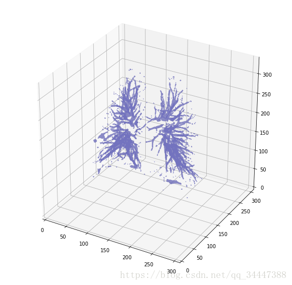
Pretty cool, no?
Anyway, when you want to use this mask, remember to first apply a dilation morphological operation on it (i.e. with a circular kernel). This expands the mask in all directions. The air + structures in the lung alone will not contain all nodules, in particular it will miss those that are stuck to the side of the lung, where they often appear! So expand the mask a little :)
This segmentation may fail for some edge cases. It relies on the fact that the air outside the patient is not connected to the air in the lungs. If the patient has a tracheostomy, this will not be the case, I do not know whether this is present in the dataset. Also, particulary noisy images (for instance due to a pacemaker in the image below) this method may also fail. Instead, the second largest air pocket in the body will be segmented. You can recognize this by checking the fraction of image that the mask corresponds to, which will be very small for this case. You can then first apply a morphological closing operation with a kernel a few mm in size to close these holes, after which it should work (or more simply, do not use the mask for this image).
很酷,是吧。对于某些边缘情况,这个分割可能会失败。原因在于病人外的空气与肺中的空气不相连。如果病人有气管造口术,情况就不是这样了,我不知道这是否存在于数据集中。另外,对于特别嘈杂的图像(例如下图有起搏器的例子)这种图像也可能失败。相反,身体中的第二大气囊将被分割。你可以通过检查mask对应的图像分数来识别这一点,在这种情况下,将非常小。然后,你可以先用一个尺寸为几毫米的内核进行形态学闭合操作,然后关闭这些孔,然后再工作(或者更简单地说,不要使用这个图像的mask)。
Normalization
Our values currently range from -1024 to around 2000. Anything above 400 is not interesting to us, as these are simply bones with different radiodensity. A commonly used set of thresholds in the LUNA16 competition to normalize between are -1000 and 400. Here's some code you can use:
归一化
值从-1024到接近2000。任何在400以上的都没啥意义,因为那些都是在不同放射线下的骨骼。在LUNA16比赛中一个普遍的用于归一化的阈值集合是-1000到400。下面是代码:
MIN_BOUND = -1000.0
MAX_BOUND = 400.0def normalize(image):image = (image - MIN_BOUND) / (MAX_BOUND - MIN_BOUND)image[image>1] = 1.image[image<0] = 0.return image
Zero centering
As a final preprocessing step, it is advisory to zero center your data so that your mean value is 0. To do this you simply subtract the mean pixel value from all pixels.
To determine this mean you simply average all images in the whole dataset. If that sounds like a lot of work, we found this to be around 0.25 in the LUNA16 competition.
Warning: Do not zero center with the mean per image (like is done in some kernels on here). The CT scanners are calibrated to return accurate HU measurements. There is no such thing as an image with lower contrast or brightness like in normal pictures.
零中心化
作为最后的预处理步骤,一个忠告——零中心化你的数据,这样数据的均值为0。要做这个,只需要减去所有像素的平均像素值即可。
确定平均像素值,你可以对整个数据集求一个平均。如果这个听起来是一个大工程量,那么可以使用我们在LUNA16比赛中发现的差不多的均值0.25。
警告:
不要以每个图像的平均值为中心。CT扫描校准,以返回准确的亨氏测量值。在正常图像中,没有像对比度或亮度一样低的图像。(然而其实不知道说的啥)
PIXEL_MEAN = 0.25def zero_center(image):image = image - PIXEL_MEANreturn imageWhat's next?
With these steps your images are ready for consumption by your CNN or other ML method :). You can do all these steps offline (one time and save the result), and I would advise you to do so and let it run overnight as it may take a long time.
Tip: To save storage space, don't do normalization and zero centering beforehand, but do this online (during training, just after loading). If you don't do this yet, your image are int16's, which are smaller than float32s and easier to compress as well.
If this tutorial helped you at all, please upvote it and leave a comment :)
下一步做什么?
经过这些步骤,你的图像已经能够送进你的卷积神经网络或其他的机器学习方法了。你能离线(也可能是能够在不进行训练的时候提前做)做这些步骤,我推荐你这样做,并且让他跑一整晚,因为它会执行很长一段时间。
建议:
为了节省存储空间,不要预先做归一化和零中心化,要在加载之后、训练的过程中做。如果你不这样做(指的就是不做预先的归一化和零中心化),你的图像是16位的int,均小于float32,易于压缩。
如果这个教程对你有帮助,请帮我点个赞并且留下个评论吧!