机器学习与高维信息检索 - Note 4 - 主成分分析及其现代解释（Principal Component Analysis, PCA）及相关实例

4. 主成分分析及其现代解释 Principal Component Analysis and Its Modern Interpretations

无监督的学习方法
输入变量是$X\in {\mathbb{R}}^n$，输出变量是还原变量$S\in {\mathbb{R}}^k$。$S$是通过某种映射$f$从$X$中计算出来的，该映射使特定的损失函数$L(f(X))$最小。无监督学习中的损失函数旨在减少 “输入变量的分布量”。这意味着$f(X)$的样本集中在一个比$X$的样本小得多的体积中。在许多情况下，这是通过做无监督的降维来实现的，即通过选择小于$n$的$k$。另外，聚类，即$S$由有限多的聚类中心组成，减少了输入分布的体积。

在所有无监督降维技术中，主成分分析（PCA）是最著名的一种。我们所说的无监督学习方法，是指在我们采用学习算法之前，数据不需要被标记（由监督者）。

PCA的成功是由于它的简单性和在许多现实世界数据分析任务中的广泛适用性。这可能是它有许多别名的原因，即离散的Karhunen-Loéve变换，Hotelling变换或适当的正交分解。它的核心假设是原始数据的分布集中在某个低维平面上，或者说，数据中的大部分方差可以通过其在这个平面上的投影方差来描述。

4.1 几何学解释

PCA的几何解释是，它通过将居中的数据投射到一个较低维度的子空间来降低维度，并用该子空间的适当的基来描述它。图4.1说明了这种解释。

我们可以将这一任务形式化如下。令$k<p$（通常是$k?p$）和$\mathbf{X}=\left[{\mathbf{x}}_1,\dots ,{\mathbf{x}}_n\right]\in$ ${\mathbb{R}}^{p\times n}$是居中的观察矩阵。回顾一下，居中的意思是 ${\sum }_i{\mathbf{x}}_i=0$。正交的${}^1$投影${\pi }_{\mathcal{U}}:{\mathbb{R}}^p\to {\mathbb{R}}^p$到$k$维的子空间$\mathcal{U}?{\mathbb{R}}^p$。可以借助$\mathcal{U}$的正交基来描述${\mathbb{R}}^p$的子集。更确切地说，如果我们用矩阵${\mathbf{U}}_k\in {\mathbb{R}}^{p\times k}$来表示这个基（即具有正交列${\mathbf{U}}_k^{?}{\mathbf{U}}_k={\mathbf{I}}_k$ )的投影由以下公式给出

$${\pi }_{\mathcal{U}}(\mathbf{x})={\mathbf{U}}_k{\mathbf{U}}_k^{?}\mathbf{x}\text{\hspace{1em}(4.1)}$$

${}^1$ 如果不做过多说明，正交总是关于标准标量的乘积。

图 4.1: PCA的几何解释：找到一个$k$维的子空间，以捕捉数据的大部分方差。第一个$\mathrm{P}\mathrm{C}$显示为红色，而第二个则显示为绿色。

因此，我们可以将任务表述为：找到一个矩阵${\mathbf{U}}_k\in {\mathbb{R}}^{p\times k}$，该矩阵具有标准正交的列，能使投影误差平方之和最小。
$$J\left({\mathbf{U}}_k\right)=\sum _{i=1}^n{\Vert {\mathbf{x}}_i?{\mathbf{U}}_k{\mathbf{U}}_k^{?}{\mathbf{x}}_i\Vert }_2^2\text{\hspace{1em}(4.2)}$$

根据下面的声明，这样的矩阵很容易找到${}^2$。

${}^2$ 我们之所以可以说这个矩阵很容易被找到，是因为在过去的几十年里，研究人员已经开发了高效可靠的算法来计算矩阵的奇异值分解。这并不意味着在一般情况下，这样的矩阵可以用手计算。

Theorem 4.1

令中心观测矩阵$\mathbf{X}$的奇异值分解为
$$\mathbf{X}={\mathbf{U}\mathbf{D}\mathbf{V}}^{?}\text{\hspace{1em}(4.3)}$$

有奇异值$d_1\ge ?\ge d_n\ge 0$。如果我们用${\mathbf{U}}_k$ 表示$\mathbf{U}$的前$k$列，那么${\mathbf{U}}_k$可以最小化（4.2）。此外，减少的$k$变量的经验协方差矩阵$\mathbf{S}:={\mathbf{U}}_k^{?}\mathbf{X}$是对角矩阵，也就是说，通过PCA提取的特征是不相关的。

---

Proof.
首先，令${\mathbf{Q}}_k\in {\mathbb{R}}^{p\times k}$ 有${\mathbf{Q}}_k^{?}{\mathbf{Q}}_k={\mathbf{I}}_k$。需要注意的是，从 ${\Vert {\mathbf{x}}_i?{\mathbf{Q}}_k{\mathbf{Q}}_k^{?}{\mathbf{x}}_i\Vert }_2^2=$ ${\Vert {\mathbf{x}}_i\Vert }_2^2?{\mathbf{x}}_i^{?}{\mathbf{Q}}_k{\mathbf{Q}}_k^{?}{\mathbf{x}}_i$开始，最小化$J$等价于 ${\sum }_i{\mathbf{x}}_i^{?}{\mathbf{Q}}_k{\mathbf{Q}}_k^{?}{\mathbf{x}}_i$。然后我们有

$$\begin{array}{rl}\sum _{i=1}^n{\mathbf{x}}_i^{?}{\mathbf{Q}}_k{\mathbf{Q}}_k^{?}{\mathbf{x}}_i& =\mathrm{tr}\left({\mathbf{Q}}_k^{?}\mathbf{X}{\mathbf{X}}^{?}{\mathbf{Q}}_k\right)\\ & =\mathrm{tr}\left({\mathbf{Q}}_k^{?}{\mathbf{U}\mathbf{D}\mathbf{D}}^{?}{\mathbf{U}}^{?}{\mathbf{Q}}_k\right)\\ & =\mathrm{tr}?{\mathbf{U}}^{?}{\mathbf{Q}}_k{\mathbf{Q}}_k^{?}{\mathbf{U}}^{?}?\begin{array}{ccc}{d}_1^2& & \\ & ?& \\ & & d_n^2\end{array}??\end{array}$$

$n\times n$ 矩阵${\mathbf{U}}^{?}{\mathbf{Q}}_k{\mathbf{Q}}_k^{?}\mathbf{U}$是一个秩为$k$的投影矩阵，因此它的对角线项都在0和1之间。为了说明这一点，让$\mathbf{P}$是一个正交投影矩阵。它的第$i$个对角线条目是 ${\mathbf{e}}_i^{?}{\mathbf{P}\mathbf{e}}_i$，其中${\mathbf{e}}_i$是第$i$个标准基向量。由于$\mathbf{P}$是一个正交的投影矩阵，我们有

$${\mathbf{e}}_i^{?}{\mathbf{P}\mathbf{e}}_i={\mathbf{e}}_i^{?}{\mathbf{P}}^2{\mathbf{e}}_i={\Vert {\mathbf{P}\mathbf{e}}_i\Vert }^2.\text{\hspace{1em}(4.4)}$$

由于$\mathbf{P}$ 是正交投影，$(\mathbf{I}?\mathbf{P})$是对正交补数的投影，${\mathbb{R}}^n$中的每个向量都可以写成投影空间中元素的唯一组合。特别是对于标准基向量来说，这一点是正确的，即

$$\begin{array}{rl}1& ={\Vert {\mathbf{e}}_i\Vert }^2={\Vert {\mathbf{P}\mathbf{e}}_i+(\mathbf{I}?\mathbf{P}){\mathbf{e}}_i\Vert }^2\\ & ={\Vert {\mathbf{P}\mathbf{e}}_i\Vert }^2+{\Vert (\mathbf{I}?\mathbf{P}){\mathbf{e}}_i\Vert }^2+2?{\mathbf{P}\mathbf{e}}_i,(\mathbf{I}?\mathbf{P}){\mathbf{e}}_i?\\ & ={\Vert {\mathbf{P}\mathbf{e}}_i\Vert }^2+{\Vert (\mathbf{I}?\mathbf{P}){\mathbf{e}}_i\Vert }^2.\end{array}\text{\hspace{1em}(4.5)}$$

由于${\mathrm{P}\mathrm{e}}_i$和$(\mathbf{I}?\mathbf{P}){\mathrm{e}}_i$是相互正交的，所以最后一个等式成立。 两个被加数${\Vert {\mathbf{P}\mathbf{e}}_i\Vert }^2$和 ${\Vert (\mathbf{I}?\mathbf{P}){\mathbf{e}}_i\Vert }^2$ 都是正数，加起来为1。因此，${\Vert {\mathbf{P}\mathbf{e}}_i\Vert }^2$ 对于所有$i$都位于$[0,1]$区间内。此外，$\mathbf{P}$的迹，即所有对角线元素之和等于$k$。因此，我们能达到的最大值是设置${\mathbf{Q}}_k={\mathbf{U}}_k$，因为此时这个投影是${\mathbf{U}}^{?}{\mathbf{U}}_k{\mathbf{U}}_k^{?}\mathbf{U}=\left[\begin{array}{cc}{\mathbf{I}}_k& 0\\ 0& 0\end{array}\right]$。

要看到还原的变量$\mathbf{S}:={\mathbf{U}}_k^{?}\mathbf{X}$是不相关的，首先注意到由于$\mathbf{X}$是居中的，所以$\mathbf{S}$也是居中的，因此它的经验协方差矩阵为

$$\mathrm{cov}(\mathbf{S}):=\frac{1}{n}{\mathbf{S}\mathbf{S}}^{?}=\frac{1}{n}{\mathbf{U}}_k^{?}{\mathbf{X}\mathbf{X}}^{?}{\mathbf{U}}_k=\frac{1}{n}?\begin{array}{lll}{d}_1^2& & \\ & ?& \\ & & d_k^2\end{array}?\text{\hspace{1em}(4.6)}$$

矩阵$\mathbf{S}$的$(i,j)$的条目称为第$i$主成分(principal component) 的第$j$得分，完整的矩阵被称为得分矩阵(score matrix) 。矩阵$\mathbf{U}$也常被称为加载矩阵(loadings matrix)。${}^3$。

${}^3$ 加载矩阵的定义在文献中并不一致。有时，矩阵$\mathbf{L}:=\mathbf{U}\mathbf{D}$被称为loading matrix，$\mathbf{U}$被表示为主轴/方向的矩阵。

注意，$\mathbf{S}$可以直接通过$\mathbf{X}$的SVD得到，因为

$$\mathbf{S}={\mathbf{U}}_k^{?}{\mathbf{U}\mathbf{D}\mathbf{V}}^{?}=?\begin{array}{ccc}{d}_1& & \\ & ?& \\ & & d_k\end{array}?{\mathbf{V}}_k^{?}={\mathbf{D}}_k{\mathbf{V}}_k^{?},\text{\hspace{1em}(4.7)}$$

其中${\mathbf{V}}_k$代表$\mathbf{V}$的前$k$列。

---

虽然减少的变量可以通过 ${\mathbf{U}}_k^{?}\mathbf{X}$来计算，但在实际应用中这是不可行的，因为${\mathbf{U}}_k$和$\mathbf{X}$都是密集的(计算S需要$(2p?1)nk$次运算)。使用${\mathbf{D}}_k{\mathbf{V}}_k^{?}$会容易很多, 因为${\mathbf{D}}_k$是对角矩阵，而${\mathbf{V}}_k^{?}$只有$k$行（计算$\mathbf{S}$需要$nk$次运算。（注，$n$为采样个数，$k$为投影后的子空间维度, $p$为原始空间维度）

4.2 统计学解释

除了最小化重建误差$J\left({\mathbf{U}}_k\right)$，如(4.2)所定义，PCA可以从统计学的角度来解释。如果$X\in {\mathbb{R}}^p$表示一个多维随机变量，PCA寻求一个正交变换到一个新的坐标系，即

$$Y={\mathbf{U}}^{?}X\text{\hspace{1em}(4.8)}$$

与${\mathbf{U}}^{?}\mathbf{U}=I_p$，这样$Y$的协方差矩阵是对角线的，而且各部分的方差都会减少，即$\mathrm{var}\left(Y_1\right)\ge ?\ge \mathrm{var}\left(Y_p\right)$。

由于协方差矩阵$\mathrm{var}(X)=\mathbb{E}\left[(X?\mu )(X?\mu {)}^{?}\right]$，其中$\mu =\mathbb{E}[X]$，是对称的正半自由度，它可以被对角化并由一个正交矩阵U排序。

$$\begin{array}{rl}\mathbf{D}& ={\mathbf{U}}^{?}\mathrm{var}(X)\mathbf{U}=\mathbb{E}\left[{\mathbf{U}}^{?}(X?\mu )(X?\mu {)}^{?}\mathbf{U}\right]\\ & =\mathbb{E}\left[\left({\mathbf{U}}^{?}X?{\mathbf{U}}^{?}\mu \right){\left({\mathbf{U}}^{?}X?{\mathbf{U}}^{?}\mu \right)}^{?}\right]=\mathrm{var}(Y)\end{array}\text{\hspace{1em}(4.9)}$$

是具有递减的正项的对角线项。如果我们考虑经验协方差矩阵，那么$\mathbf{U}$由居中观测矩阵的SVD给出，作为 左奇异向量，参见（4.3）。

4.3 误差模型解释 （Error Model Interpretation）

把观察到的数据$\mathbf{X}$看作是位于某个$k$维子空间的一些干净数据$\mathbf{L}$和一些额外的噪声$\mathbf{N}$的叠加，即

$$\mathbf{X}=\mathbf{L}+\mathbf{N}\text{\hspace{1em}(4.10)}$$

从形式上看，要求$\mathbf{L}$的数据位于某个$k$维的子空间中，相当于要求$\mathbf{L}$的等级低于或等于$k$。我们将在下文中看到，看待PCA的另一种方式是我们要恢复$\mathbf{L}$，在噪声$\mathbf{N}$（从各个项来看）是各自独立的高斯分布的情况下。其中噪声矩阵$\mathbf{N}$的每个条目是根据均值为0、方差为1的高斯分布独立抽取的。在这种模型假设下，给定观测值$\mathbf{X}$的最大似然估计$\mathbf{L}$为，

$$\hat{\mathbf{L}}=\arg \underset{\text{rank }\mathbf{L}\le k}{\min }\Vert \mathbf{X}?\mathbf{L}{\Vert }_F\text{. }\text{\hspace{1em}(4.11)}$$

经典的PCA提供了这个问题的解决方案。

Theorem 4.2.

设$\mathbf{X}={\mathbf{U}\mathbf{D}\mathbf{V}}^{?}$为观察矩阵$\mathbf{X}$的奇异值分解，奇异值为$d_1\ge ?\ge d_p\ge 0$。如果我们用${\mathbf{U}}_k$表示$\mathbf{U}$的前$k$列，用${\mathbf{V}}_k$表示$\mathbf{V}$的前$k$列，那么$\hat{\mathbf{L}}={\mathbf{U}}_k\mathrm{diag}\left(d_1,\dots ,d_k\right){\mathbf{V}}_k^{?}$ 最小化(4.11)。

---

Proof.

让$\mathbf{L}$是(4.11)的最小化。请注意，矩阵$\mathbf{L}$的秩低于或等于$k$，当且仅当其列${\mathbf{l}}_i$位于$k$维的子空间中，例如$\mathcal{L}$。现在每一列${\mathbf{I}}_i$必须是${\mathbf{x}}_i$对$\mathcal{L}$的投影，否则，我们可以在不增加$|\mathbf{X}?\mathbf{L}{\Vert }_F^2={\sum }_i{|{\mathbf{x}}_i?1_i\Vert }^2$的情况下取代$\mathbf{L}$矩阵的第$i$列。因此

$$\underset{\mathrm{r}\mathrm{k}\mathrm{L}\le k}{\min }\Vert \mathbf{X}?\mathbf{L}{\Vert }_F^2=\underset{\dim (\mathcal{L})=k}{\min }\sum _i{\Vert {\mathbf{x}}_i?{\pi }_{\mathcal{L}}\left({\mathbf{x}}_i\right)\Vert }^2,\text{\hspace{1em}(4.12)}$$

从定理4.1可以看出，$\mathcal{L}$由$\mathbf{X}$的前$k$奇异向量${\mathbf{U}}_k$所张成，因此最佳$k$-秩近似值为

$$\hat{\mathbf{L}}={\mathbf{U}}_k{\mathbf{U}}_k^{?}\mathbf{X}={\mathbf{U}}_k\mathrm{diag}\left(d_1,\dots ,d_k\right){\mathbf{V}}_k^{?}\text{\hspace{1em}(4.13)}$$

4.4 Relation to Autoencoders

PCA与一种特别简单的神经网络形式密切相关，即所谓的自动编码器。自动编码器的目的是在输入通过一个低维空间后尽可能好地重建输入，或者更正式地说。$p$维随机变量的实现$x_1,\dots ,x_n$首先通过函数$f$被映射到低维空间${\mathbb{R}}^k$，然后这些图像再次被映射到${\mathbb{R}}^p$，试图最适合原始输入。

$$g?f\left({\mathbf{x}}_i\right)\approx {\mathbf{x}}_i.\text{\hspace{1em}(4.14)}$$

自动编码器试图为这项工作找到最佳的一对函数$(f,g)$，其想法是，有趣信息的合理部分包含在减少的数据$f\left({\mathbf{x}}_i\right)$中。现在让我们假设$f$和$g$是线性的，由矩阵$\mathbf{V}\in {\mathbb{R}}^{k\times p}$ 与$\mathbf{W}\in {\mathbb{R}}^{p\times k}$ 。那么$g?f\left({\mathbf{x}}_i\right)=\mathbf{W}\mathbf{V}{\mathbf{x}}_i$，如果我们通过平方距离之和来测量重建误差，即

$$J(\mathbf{W},\mathbf{V})=\sum _{i=1}^n{\Vert {\mathbf{x}}_i?\mathbf{W}\mathbf{V}{\mathbf{x}}_i\Vert }^2\text{\hspace{1em}(4.15)}$$

我们可以证明，最优的$\mathbf{V}$只是由观察矩阵$\mathbf{X}=\left[{\mathbf{x}}_1,\dots ,{\mathbf{x}}_n\right]$的前$k$左奇异向量给出。

Theorem 4.3

设${\mathbf{U}}_k$为观察矩阵$\mathbf{X}$的前$k$左奇异向量。那么$\mathbf{V}={\mathbf{U}}_k^{?}$和$\mathbf{W}={\mathbf{U}}_k$使线性编码器的重建误差最小（4.15）。

---

Proof.
由于$\mathbf{V}$和$\mathbf{W}$的维数，平方矩阵$\mathbf{W}\mathbf{V}$最多可以有$k$的秩。所以，所有$\mathbf{W}\mathbf{V}{\mathbf{x}}_i$位于一个$k$维的子空间中，因此形成一个最多秩为$k$的矩阵。我们在定理4.2中看到，$L$的最小值是由$\mathbf{V}={\mathbf{U}}_k^{?}$和$\mathbf{W}={\mathbf{U}}_k$实现。

通过允许非线性函数，这种方法有了有趣的扩展。在实际应用中非常成功的是$f(\mathbf{x}):=\sigma (\mathbf{V}\mathbf{x})$形式的函数，其中$\mathbf{V}$是上述情况下的矩阵，$\sigma$是一个激活函数，分量操作，对负参数为零，对正参数不做改变。在这种非线性设置中，所产生的优化问题没有封闭式的解决方案，我们需要优化技术，例如梯度下降法，来近似地获得一个最佳解决方案。

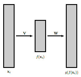
图4.2：一个简单的自动编码器，有 $\mathbf{V}\in {\mathbb{R}}^{k\times p},\mathbf{W}\in {\mathbb{R}}^{p\times k},k<p$。

4.5 PCA 实例

Task 1.

In this task, we will once again work with the MNIST training set as provided on Moodle. Choose three digit classes, e.g. 1,2 and 3 and load $N=1000$ images from each of the classes to the workspace. Store the data in a floating point matrix $X$ of shape $(784,3?\mathrm{N})$ normalized to the number range $[0,1]$. Furthermore, generate a color label matrix C of dimensions $(3?N,3)$ . Each row of C assigns an RGB color vector to the respective column of $X$ as an indicator of the digit class. Choose $[0,0,1],[0,1,0]$ and $[1,0,0]$ for the three digit classes.

a) Compute the row-wise mean mu of $X$ and subtract it from each column of $X$ . Save the results as $X_c$.

b) Use np. linalg.svd with full_matrices=False to compute the singular value decomposition $[U,Sigma,VT]$ of $X_C$ . Make sure the matrices are sorted in descending order with respect to the singular values.

c) Use reshape in order to convert mu and the first three columns of U to (28,28) -matrices. Plot the resulting images. What do you see?

d) Compute the matrix $S=np?\mathrm{dot}(np?\mathrm{diag}(Sigma),VT)$ . Note that this yields the same result as $S=np?\mathrm{dot}\left(U?T,X_{?}C\right)$ . The S matrix contains the $3?\mathrm{N}$ scores for the principal components 1 to 784 . Create a 2D scatter plot with C as its color parameter in order to plot the scores for the first two principal components of the data.

import numpy as np
import matplotlib.pyplot as pltimport imageio# define to image paths which to import
data_folder = './mnist/'
N = 1000
X = np.zeros((784, 3 * N))for n in range(N):# define the images' pathimpath0 = data_folder + 'd1/d1_{}.png'.format(str(n + 1).zfill(4))impath1 = data_folder + 'd2/d2_{}.png'.format(str(n + 1).zfill(4))impath2 = data_folder + 'd3/d3_{}.png'.format(str(n + 1).zfill(4))# import and convert to numpy arrayI0 = np.array(imageio.imread(impath0)).astype(np.float64).reshape(784, ) / 255I1 = np.array(imageio.imread(impath1)).astype(np.float64).reshape(784, ) / 255I2 = np.array(imageio.imread(impath2)).astype(np.float64).reshape(784, ) / 255X[:, n] = I0X[:, n + N] = I1X[:, n + 2 * N] = I2C = np.zeros((3 * N, 3))
C[0:N, :] = [0, 0, 1]
C[N:2 * N, :] = [0, 1, 0]
C[2 * N:3 * N, :] = [1, 0, 0]mu = np.mean(X, axis=1)
X_c = X - np.expand_dims(np.mean(X, axis=1), axis=1) \\
# singular decomposition
[U, Sigma, VT] = np.linalg.svd(X_c, full_matrices=False)# the resulting images
plt.figure(1)
plt.subplot(1, 4, 1)
plt.title('mu')
plt.imshow(mu[:, ].reshape(28, 28))
for n in range(3):plt.subplot(1, 4, n + 2)plt.title('U[:, {}]'.format(n))plt.imshow(U[:, n].reshape(28, 28))
plt.show()# calculate the projection
S = np.dot(np.diag(Sigma), VT)  # Using Sigma*V.T is more efficientidx_new = np.arange(3 * N).reshape(3, N).T.ravel()plt.figure(2)
# using the first two features to scatter the points,
# the parameters are (feature 1, feature 2, color) of a specific point
plt.scatter(S[0, idx_new], S[1, idx_new], c=C[idx_new])
plt.show()

the outputs are,

Task 2.

In this task, we consider the problem of choosing the number of principal vectors. Assuming that $\mathbf{X}\in {\mathbb{R}}^{p\times N}$ is the centered data matrix and $\mathbf{P}={\mathbf{U}}_k{\mathbf{U}}_k^{?}$ is the projector onto the k -dimensional principal subspace, the dimension $k$ is chosen such that the fraction of overall energy contained in the projection error does not exceed $?$ , i.e.

$$\frac{\Vert \mathbf{X}?\mathbf{P}\mathbf{X}{\Vert }_F^2}{\Vert \mathbf{X}{\Vert }_F^2}=\frac{{\sum }_{i=1}^M{\Vert {\mathbf{x}}_i?\mathbf{P}{\mathbf{x}}_i\Vert }^2}{{\sum }_{i=1}^N{\Vert {\mathbf{x}}_i\Vert }^2}\le ?$$

where $?$ is usually chosen to be between 0.01 and 0.2 .

The MIT VisTex database consists of a set of 167 RGB texture images of sizes (512,512,3) .

a) After preprocessing the entire image set (converting to normalized grayscale matrices), divide the images into non overlapping tiles of sizes (64,64) and create a centered data matrix X_c of size $(p,N)$ from them, where p=64*64 and N=167 *(512 / 64) *(512 / 64) .

b) Compute the SVD of X_c and make sure the singular values are sorted in descending order.

c) Plot the fraction of signal energy contained in the projection error for the principal subspace dimensions 0 to p. How many principal vectors do you need to retain 80%, 90%, 95 % or 99 % of the original signal energy?

d) Discuss: Can you imagine a scenario, where signal energy is a bad measure of useful information?

import os, glob
import matplotlib.pyplot as plt
import imageio
import numpy as npdef rgb2gray(rgb):r, g, b = rgb[:,:,0], rgb[:,:,1], rgb[:,:,2]gray = 0.2989 * r + 0.5870 * g + 0.1140 * breturn grayif __name__ == '__main__':# define data directorydata_dir = 'VisTex_512_512'# change to correct directoryfiles = glob.glob(data_dir+'/*.ppm')# define number of filesimg_N = len(files)p = 64 * 64  # tiles sizeN = np.uint16(167 * (512/64) * (512/64))  # Number of tilesX = np.zeros((p, N))for f in range(img_N):img = imageio.imread(files[f])img = rgb2gray(np.array(img)/255.0)for k in range(0, 8):for j in range(0, 8):x_tmp = img[k*64:(k+1)*64, j*64:(j+1)*64].ravel()X[:, np.uint16(f*(512/64)**2 + k*8 + j)] = x_tmp# a) centered data matrixmu = np.mean(X, axis=1)X_c = X - np.expand_dims(mu, 1)# b) the SVD of X_c[U, Sigma, VT] = np.linalg.svd(X_c, full_matrices=False)  # full_matrices?[U_x, Sigma_x, VT_x] = np.linalg.svd(X, full_matrices=False)# c) the preserved energy'''Remark : Sigma can be described the values which contains the energy of each subspace. If we accumulate all sigma, then we can get the whole energy of the original matrix.'''p_steps = np.arange(p+1)proj_error = np.array([(1.0 - np.sum(Sigma[:i]**2)/np.sum(Sigma**2))*100.0 for i in p_steps])plt.plot(p_steps, proj_error)plt.xlabel('Dimension'); plt.ylabel('Projection Error (%)')plt.show()print('Required dimension of subspace for Preservation of 80% of the energy:', np.sum(np.uint16(proj_error>=20))+1)print('Required dimension of subspace for Preservation of 90% of the energy:', np.sum(np.uint16(proj_error>=10))+1)print('Required dimension of subspace for Preservation of 95% of the energy:', np.sum(np.uint16(proj_error>=5))+1)print('Required dimension of subspace for Preservation of 99% of the energy:', np.sum(np.uint16(proj_error>=1))+1)proj_error_x = np.array([(1.0-np.sum(Sigma_x[:i]**2)/np.sum(Sigma_x**2))*100.0 for i in p_steps])plt.plot(p_steps, proj_error_x)plt.xlabel('Dimension'); plt.ylabel('Projection Error (%)')plt.show()print('Required dimension of subspace for Preservation of 80% of the energy:', np.sum(np.uint16(proj_error_x>=20))+1)print('Required dimension of subspace for Preservation of 90% of the energy:', np.sum(np.uint16(proj_error_x>=10))+1)print('Required dimension of subspace for Preservation of 95% of the energy:', np.sum(np.uint16(proj_error_x>=5))+1)print('Required dimension of subspace for Preservation of 99% of the energy:', np.sum(np.uint16(proj_error_x>=1))+1)

Using the centered observation matrix:
Required dimension of subspace for Preservation of 80% of the energy: 98
Required dimension of subspace for Preservation of 90% of the energy: 335
Required dimension of subspace for Preservation of 95% of the energy: 694
Required dimension of subspace for Preservation of 99% of the energy: 1651Without the centered observation matrix:
Required dimension of subspace for Preservation of 80% of the energy: 2
Required dimension of subspace for Preservation of 90% of the energy: 17
Required dimension of subspace for Preservation of 95% of the energy: 121
Required dimension of subspace for Preservation of 99% of the energy: 877

the outputs are,

d)

A typical situation that arises with machine learning on natural images is that lighting conditions vary heavily. Often, the overall brightness of a picture does not add any discriminative value to it. For instance, a face recognition system should not care about whether a picture was taken at day or at night. However, if the overall brighness varies over a set of images that is processed by PCA, the first principal components will mostly contain the brightness information.

$$\begin{array}{rl}\hat{\mathrm{s}}& =\underset{\mathrm{s}\text{ s.t. }\Vert \mathrm{s}\Vert =1}{\mathrm{argmax}}{\mathrm{s}}^{?}\Sigma {\Sigma }^{?}\mathrm{s}\\ & =\underset{\mathrm{s}\text{ s.t. }\Vert \mathrm{s}\Vert =1}{\mathrm{argmax}}||\mathrm{s}\Sigma |{|}^2\\ & =\underset{\mathrm{s}\text{ s.t. }\Vert \mathrm{s}\Vert =1}{\mathrm{argmax}}||\mathrm{s}\mathrm{diag}({\sigma }_{1,1},...,{\sigma }_{p,p})|{|}^2\end{array}$$

$$\hat{\mathrm{s}}=\underset{\mathrm{s}\text{ s.t. }\Vert \mathrm{s}\Vert =1}{\mathrm{argmax}}{\mathrm{s}}^{?}\Sigma {\Sigma }^{?}\mathrm{s}$$.