数据分析――阿里资金流入流出分析(task1-数据探索与分析)
学习目标
熟悉数据分析的流程,了解金融时间序列分析的一般方法。
任务安排
数据集可在阿里天池下载:
https://tianchi.aliyun.com/competition/entrance/231573/information
数据实践
库导入
import pandas as  pd
import numpy as np
import warnings
import datetime
import seaborn as sns
import matplotlib.pyplot as plt
import datetime
from scipy import statsimport warnings
warnings.filterwarnings('ignore')# 设置数据集路径dataset_path = 'Dataset/'# 读取数据data_balance = pd.read_csv(dataset_path+'user_balance_table.csv')# 为数据集添加时间戳data_balance['date'] = pd.to_datetime(data_balance['report_date'], format= "%Y%m%d")
data_balance['day'] = data_balance['date'].dt.day
data_balance['month'] = data_balance['date'].dt.month
data_balance['year'] = data_balance['date'].dt.year
data_balance['week'] = data_balance['date'].dt.week
data_balance['weekday'] = data_balance['date'].dt.weekday
一、时间序列分析
# 聚合时间数据total_balance = data_balance.groupby(['date'])['total_purchase_amt','total_redeem_amt'].sum().reset_index()
# 生成测试集区段数据start = datetime.datetime(2014,9,1)
testdata = []
while start != datetime.datetime(2014,10,1):temp = [start, np.nan, np.nan]testdata.append(temp)start += datetime.timedelta(days = 1)
testdata = pd.DataFrame(testdata)
testdata.columns = total_balance.columns# 拼接数据集total_balance = pd.concat([total_balance, testdata], axis = 0)# 为数据集添加时间戳total_balance['day'] = total_balance['date'].dt.day
total_balance['month'] = total_balance['date'].dt.month
total_balance['year'] = total_balance['date'].dt.year
total_balance['week'] = total_balance['date'].dt.week
total_balance['weekday'] = total_balance['date'].dt.weekday
import matplotlib.pylab as plt
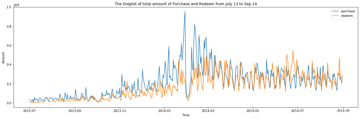
# 画出每日总购买与赎回量的时间序列图fig = plt.figure(figsize=(20,6))
plt.plot(total_balance['date'], total_balance['total_purchase_amt'],label='purchase')
plt.plot(total_balance['date'], total_balance['total_redeem_amt'],label='redeem')plt.legend(loc='best')
plt.title("The lineplot of total amount of Purchase and Redeem from July.13 to Sep.14")
plt.xlabel("Time")
plt.ylabel("Amount")
plt.show()
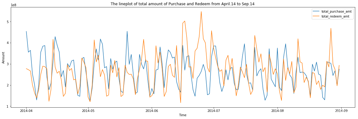
# 画出4月份以后的时间序列图total_balance_1 = total_balance[total_balance['date'] >= datetime.date(2014,4,1)]
fig = plt.figure(figsize=(20,6))
plt.plot(total_balance_1['date'], total_balance_1['total_purchase_amt'])
plt.plot(total_balance_1['date'], total_balance_1['total_redeem_amt'])
plt.legend()
plt.title("The lineplot of total amount of Purchase and Redeem from April.14 to Sep.14")
plt.xlabel("Time")
plt.ylabel("Amount")
plt.show()
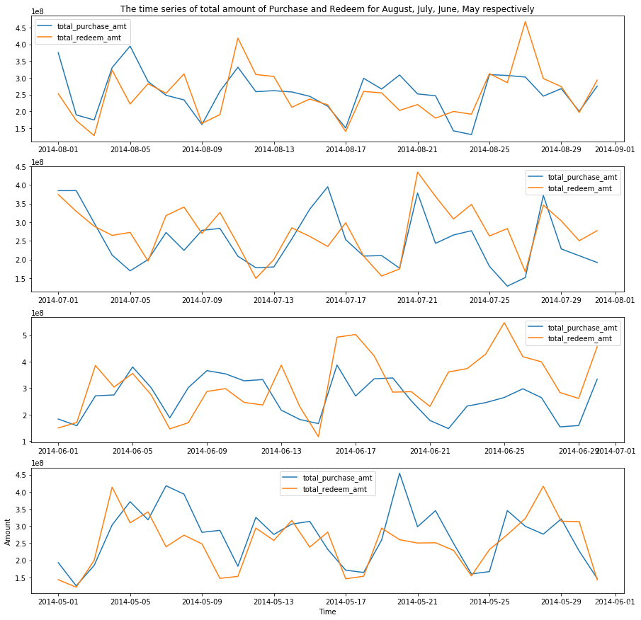
# 分别画出每个月中每天购买赎回量的时间序列图fig = plt.figure(figsize=(15,15))plt.subplot(4,1,1)
plt.title("The time series of total amount of Purchase and Redeem for August, July, June, May respectively")total_balance_2 = total_balance[total_balance['date'] >= datetime.date(2014,8,1)]
plt.plot(total_balance_2['date'], total_balance_2['total_purchase_amt'])
plt.plot(total_balance_2['date'], total_balance_2['total_redeem_amt'])
plt.legend()total_balance_3 = total_balance[(total_balance['date'] >= datetime.date(2014,7,1)) & (total_balance['date'] < datetime.date(2014,8,1))]
plt.subplot(4,1,2)
plt.plot(total_balance_3['date'], total_balance_3['total_purchase_amt'])
plt.plot(total_balance_3['date'], total_balance_3['total_redeem_amt'])
plt.legend()total_balance_4 = total_balance[(total_balance['date'] >= datetime.date(2014,6,1)) & (total_balance['date'] < datetime.date(2014,7,1))]
plt.subplot(4,1,3)
plt.plot(total_balance_4['date'], total_balance_4['total_purchase_amt'])
plt.plot(total_balance_4['date'], total_balance_4['total_redeem_amt'])
plt.legend()total_balance_5 = total_balance[(total_balance['date'] >= datetime.date(2014,5,1)) & (total_balance['date'] < datetime.date(2014,6,1))]
plt.subplot(4,1,4)
plt.plot(total_balance_5['date'], total_balance_5['total_purchase_amt'])
plt.plot(total_balance_5['date'], total_balance_5['total_redeem_amt'])
plt.legend()plt.xlabel("Time")
plt.ylabel("Amount")
plt.show()
# 分别画出13年8月与9月每日购买赎回量的时序图fig = plt.figure(figsize=(15,9))total_balance_last8 = total_balance[(total_balance['date'] >= datetime.date(2013,8,1)) & (total_balance['date'] < datetime.date(2013,9,1))]
plt.subplot(2,1,1)
plt.plot(total_balance_last8['date'], total_balance_last8['total_purchase_amt'])
plt.plot(total_balance_last8['date'], total_balance_last8['total_redeem_amt'])
plt.legend()total_balance_last9 = total_balance[(total_balance['date'] >= datetime.date(2013,9,1)) & (total_balance['date'] < datetime.date(2013,10,1))]
plt.subplot(2,1,2)
plt.plot(total_balance_last9['date'], total_balance_last9['total_purchase_amt'])
plt.plot(total_balance_last9['date'], total_balance_last9['total_redeem_amt'])
plt.legend()plt.xlabel("Time")
plt.ylabel("Amount")
plt.show()

二、翌日特征分析
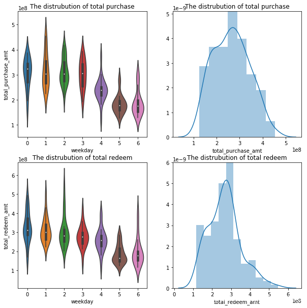
# 画出每个翌日的数据分布于整体数据的分布图a = plt.figure(figsize=(10,10))
scatter_para = {'marker':'.', 's':3, 'alpha':0.3}
line_kws = {'color':'k'}
plt.subplot(2,2,1)
plt.title('The distrubution of total purchase')
sns.violinplot(x='weekday', y='total_purchase_amt', data = total_balance_1, scatter_kws=scatter_para, line_kws=line_kws)
plt.subplot(2,2,2)
plt.title('The distrubution of total purchase')
sns.distplot(total_balance_1['total_purchase_amt'].dropna())
plt.subplot(2,2,3)
plt.title('The distrubution of total redeem')
sns.violinplot(x='weekday', y='total_redeem_amt', data = total_balance_1, scatter_kws=scatter_para, line_kws=line_kws)
plt.subplot(2,2,4)
plt.title('The distrubution of total redeem')
sns.distplot(total_balance_1['total_redeem_amt'].dropna())
# 按翌日对数据聚合后取均值week_sta = total_balance_1[['total_purchase_amt', 'total_redeem_amt', 'weekday']].groupby('weekday', as_index=False).mean()# 分析翌日的中位数特征plt.figure(figsize=(12, 5))
ax = plt.subplot(1,2,1)
plt.title('The barplot of average total purchase with each weekday')
ax = sns.barplot(x="weekday", y="total_purchase_amt", data=week_sta, label='Purchase')
ax.legend()
ax = plt.subplot(1,2,2)
plt.title('The barplot of average total redeem with each weekday')
ax = sns.barplot(x="weekday", y="total_redeem_amt", data=week_sta, label='Redeem')
ax.legend()

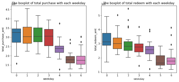
# 画出翌日的箱型图plt.figure(figsize=(12, 5))
ax = plt.subplot(1,2,1)
plt.title('The boxplot of total purchase with each weekday')
ax = sns.boxplot(x="weekday", y="total_purchase_amt", data=total_balance_1)
ax = plt.subplot(1,2,2)
plt.title('The boxplot of total redeem with each weekday')
ax = sns.boxplot(x="weekday", y="total_redeem_amt", data=total_balance_1)
# 使用OneHot方法将翌日特征划分,获取划分后特征from sklearn.preprocessing import OneHotEncoder
encoder = OneHotEncoder()
total_balance = total_balance.reset_index()
week_feature = encoder.fit_transform(np.array(total_balance['weekday']).reshape(-1, 1)).toarray()
week_feature = pd.DataFrame(week_feature,columns=['weekday_onehot']*len(week_feature[0]))
feature = pd.concat([total_balance, week_feature], axis = 1)[['total_purchase_amt', 'total_redeem_amt','weekday_onehot','date']]
feature.columns = list(feature.columns[0:2]) + [x+str(i) for i,x in enumerate(feature.columns[2:-1])] + ['date']
# 画出划分后翌日特征与标签的斯皮尔曼相关性f, ax = plt.subplots(figsize = (15, 8))
plt.subplot(1,2,1)
plt.title('The spearman coleration between total purchase and each weekday')
sns.heatmap(feature[[x for x in feature.columns if x not in ['total_redeem_amt', 'date'] ]].corr('spearman'),linewidths = 0.1, vmax = 0.2, vmin=-0.2)
plt.subplot(1,2,2)
plt.title('The spearman coleration between total redeem and each weekday')
sns.heatmap(feature[[x for x in feature.columns if x not in ['total_purchase_amt', 'date'] ]].corr('spearman'),linewidths = 0.1,  vmax = 0.2, vmin=-0.2)

# 测试翌日特征与标签的独立性 Ref: https://github.com/ChuanyuXue/MVTestfrom mvtpy.mvtest import mvtest
mv = mvtest()
mv.test(total_balance_1['total_purchase_amt'], total_balance_1['weekday'])
{'Tn': 6.75, 'p-value': [0, 0.01]}
三、月份特征分析
# 画出每个月的购买总量分布估计图(kdeplot)plt.figure(figsize=(15,10))
plt.title('The Probability Density of total purchase amount in Each Month')
plt.ylabel('Probability')
plt.xlabel('Amount')
for i in range(7, 12):sns.kdeplot(total_balance[(total_balance['date'] >= datetime.date(2013,i,1)) & (total_balance['date'] < datetime.date(2013,i+1,1))]['total_purchase_amt'],label='13Y,'+str(i)+'M')
for i in range(1, 9):sns.kdeplot(total_balance[(total_balance['date'] >= datetime.date(2014,i,1)) & (total_balance['date'] < datetime.date(2014,i+1,1))]['total_purchase_amt'],label='14Y,'+str(i)+'M')

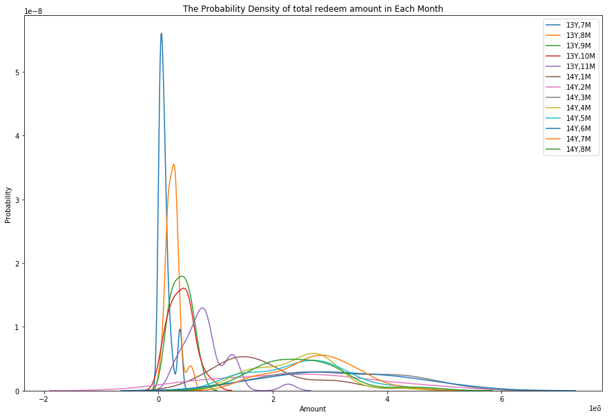
# 画出每个月的赎回总量分布估计图(kdeplot)plt.figure(figsize=(15,10))
plt.title('The Probability Density of total redeem amount in Each Month')
plt.ylabel('Probability')
plt.xlabel('Amount')
for i in range(7, 12):sns.kdeplot(total_balance[(total_balance['date'] >= datetime.date(2013,i,1)) & (total_balance['date'] < datetime.date(2013,i+1,1))]['total_redeem_amt'],label='13Y,'+str(i)+'M')
for i in range(1, 9):sns.kdeplot(total_balance[(total_balance['date'] >= datetime.date(2014,i,1)) & (total_balance['date'] < datetime.date(2014,i+1,1))]['total_redeem_amt'],label='14Y,'+str(i)+'M')
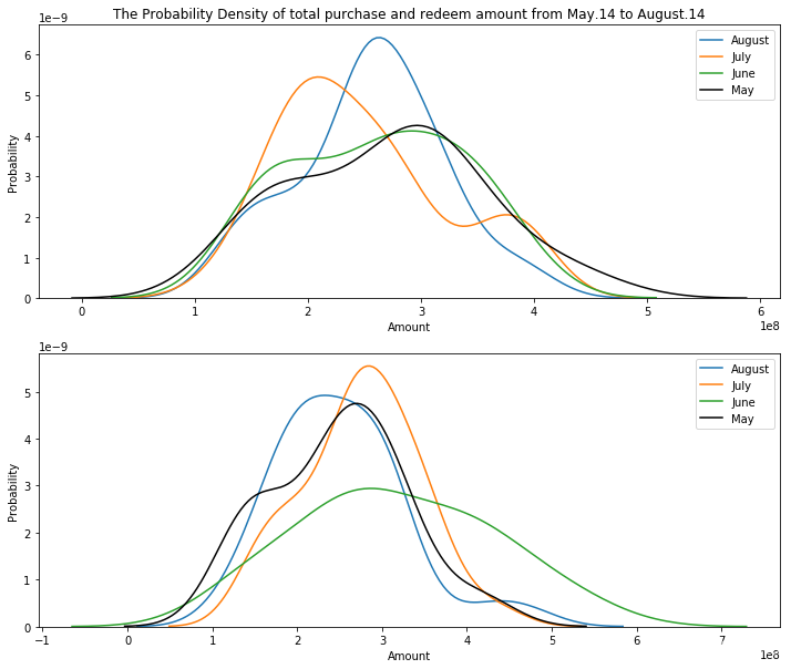
# 画出14年五六七八月份的分布估计图plt.figure(figsize=(12,10))ax = plt.subplot(2,1,1)
plt.title('The Probability Density of total purchase and redeem amount from May.14 to August.14')
plt.ylabel('Probability')
plt.xlabel('Amount')
ax = sns.kdeplot(total_balance_2['total_purchase_amt'],label='August')
ax = sns.kdeplot(total_balance_3['total_purchase_amt'],label='July')
ax = sns.kdeplot(total_balance_4['total_purchase_amt'],label='June')
ax = sns.kdeplot(total_balance_5['total_purchase_amt'],color='Black',label='May')
ax = plt.subplot(2,1,2)
plt.ylabel('Probability')
plt.xlabel('Amount')
ax = sns.kdeplot(total_balance_2['total_redeem_amt'],label='August')
ax = sns.kdeplot(total_balance_3['total_redeem_amt'],label='July')
ax = sns.kdeplot(total_balance_4['total_redeem_amt'],label='June')
ax = sns.kdeplot(total_balance_5['total_redeem_amt'],color='Black',label='May')
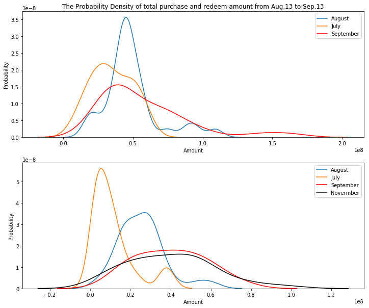
# 画出13年八月到九月份的分布估计图total_balance_last_7 = total_balance[(total_balance['date'] >= datetime.date(2013,7,1)) & (total_balance['date'] < datetime.date(2013,8,1))]
total_balance_last_8 = total_balance[(total_balance['date'] >= datetime.date(2013,8,1)) & (total_balance['date'] < datetime.date(2013,9,1))]
total_balance_last_9 = total_balance[(total_balance['date'] >= datetime.date(2013,9,1)) & (total_balance['date'] < datetime.date(2013,10,1))]
total_balance_last_10 = total_balance[(total_balance['date'] >= datetime.date(2013,10,1)) & (total_balance['date'] < datetime.date(2013,11,1))]
plt.figure(figsize=(12,10))
ax = plt.subplot(2,1,1)
plt.title('The Probability Density of total purchase and redeem amount from Aug.13 to Sep.13')
plt.ylabel('Probability')
plt.xlabel('Amount')
ax = sns.kdeplot(total_balance_last_8['total_purchase_amt'],label='August')
ax = sns.kdeplot(total_balance_last_7['total_purchase_amt'],label='July')
ax = sns.kdeplot(total_balance_last_9['total_purchase_amt'],color='Red',label='September')ax = plt.subplot(2,1,2)
plt.ylabel('Probability')
plt.xlabel('Amount')
ax = sns.kdeplot(total_balance_last_8['total_redeem_amt'],label='August')
ax = sns.kdeplot(total_balance_last_7['total_redeem_amt'],label='July')
ax = sns.kdeplot(total_balance_last_9['total_redeem_amt'],color='Red',label='September')
ax = sns.kdeplot(total_balance_last_10['total_redeem_amt'],color='Black',label='Novermber')
四、日期特征分析
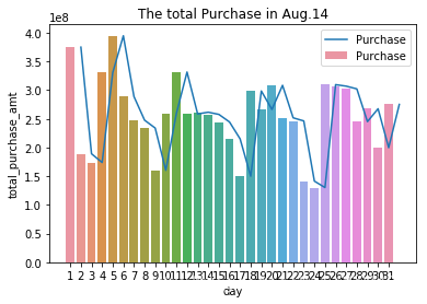
# 按照每天聚合数据集day_sta = total_balance_2[['total_purchase_amt', 'total_redeem_amt', 'day']].groupby('day', as_index=False).mean()# 获取聚合后每月购买分布的柱状图ax = sns.barplot(x="day", y="total_purchase_amt", data=day_sta, label='Purchase')
ax = sns.lineplot(x="day", y="total_purchase_amt", data=day_sta, label='Purchase')
ax.legend()
plt.title("The total Purchase in Aug.14")
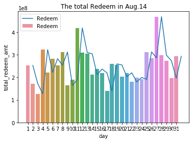
# 获取聚合后每月赎回分布的柱状图ax = sns.barplot(x="day", y="total_redeem_amt", data=day_sta, label='Redeem')
ax = sns.lineplot(x="day", y="total_redeem_amt", data=day_sta, label='Redeem')
ax.legend()
plt.title("The total Redeem in Aug.14")
# 画出13年九月份的分布图plt.figure(figsize=(15,5))
day_sta = total_balance_last_9[['total_purchase_amt', 'total_redeem_amt', 'day']].groupby('day', as_index=False).mean()
plt.subplot(1,2,1)
plt.title("The total Purchase in Sep.13")
ax = sns.barplot(x="day", y="total_purchase_amt", data=day_sta, label='Purchase')
ax = sns.lineplot(x="day", y="total_purchase_amt", data=day_sta, label='Purchase')
plt.subplot(1,2,2)
plt.title("The total Redeem in Sep.13")
bx = sns.barplot(x="day", y="total_redeem_amt", data=day_sta, label='Redeem')
bx = sns.lineplot(x="day", y="total_redeem_amt", data=day_sta, label='Redeem')
bx.legend()

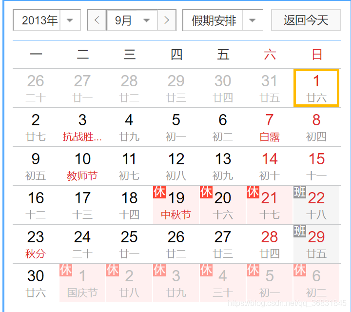
We find that the data from last year in Sep has very limited week feature
There are some strange day in Sep:
- 1st day
- 2nd day
- 16th day(Purchase a lot)―Monday & 3days before MidAutumn Festirval
- 11th day and 25th day(Redeem a lot)―Both of Wednesday
- 18 19 20(Both Purchase and Redeem is very low)
# 画出历史所有天的热力图test = np.zeros((max(total_balance_1['week']) - min(total_balance_1['week']) + 1, 7))
test[total_balance_1['week'] - min(total_balance_1['week']), total_balance_1['weekday']] = total_balance_1['total_purchase_amt']f, ax = plt.subplots(figsize = (10, 4))
sns.heatmap(test,linewidths = 0.1, ax=ax)
ax.set_title("Purchase")
ax.set_xlabel('weekday')
ax.set_ylabel('week')test = np.zeros((max(total_balance_1['week']) - min(total_balance_1['week']) + 1, 7))
test[total_balance_1['week'] - min(total_balance_1['week']), total_balance_1['weekday']] = total_balance_1['total_redeem_amt']f, ax = plt.subplots(figsize = (10, 4))
sns.heatmap(test,linewidths = 0.1, ax=ax)
ax.set_title("Redeem")
ax.set_xlabel('weekday')
ax.set_ylabel('week')
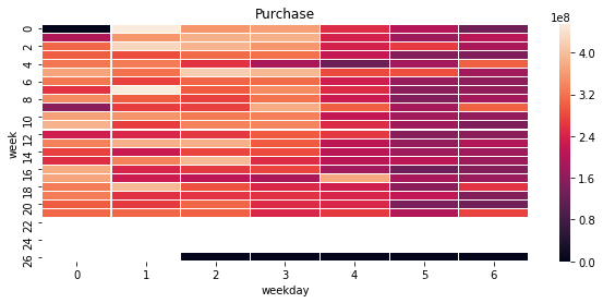
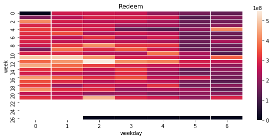
From the heat map we find that the data of week 4 and weekday 6 is very strange, and week 12 weekday 2 either
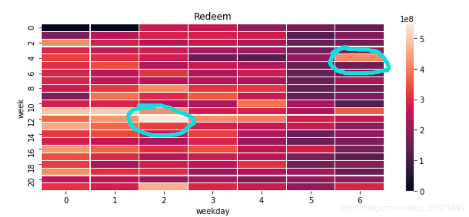
# 对于热力图中异常点的数据分析.1total_balance_1[(total_balance_1['week'] == 4 + min(total_balance_1['week'])) & (total_balance_1['weekday'] == 6)]
date	total_purchase_amt	total_redeem_amt	day	month	year	week	weekday
307	2014-05-04	303087562.0	413222034.0	4	5	2014	18	6
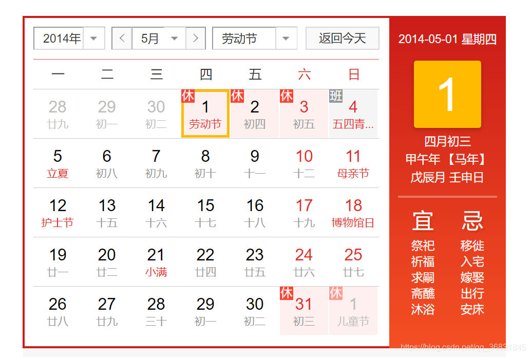
2014-5-4 is a special day in China, It is the first workday after the Labour day!
# 对于热力图中异常点的数据分析.2total_balance_1[(total_balance_1['week'] == 12 + min(total_balance_1['week'])) & (total_balance_1['weekday'] == 2)]
date	total_purchase_amt	total_redeem_amt	day	month	year	week	weekday
359	2014-06-25	264663201.0	547295931.0	25	6	2014	26	2


五、对于节假期的分析
- The QingMing festerval (April.5 - April.7)
- The Labour day (May.1 - May.5)
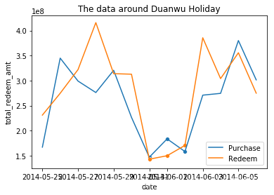
- The DuanWu festeval (May.31 - June.2)
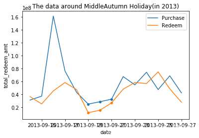
- The MidAutumn festeval (Sep.6 - Sep.8)
Others - Mother day(May.13)
- Father day(June. 17)
- TianMao 618 sales(June 10 - June 20)
- Teachers’ day(Sep 9)
# 获取节假日的数据qingming = total_balance[(total_balance['date'] >= datetime.date(2014,4,5)) & (total_balance['date'] < datetime.date(2014,4,8))]
labour = total_balance[(total_balance['date'] >= datetime.date(2014,5,1)) & (total_balance['date'] < datetime.date(2014,5,4))]
duanwu = total_balance[(total_balance['date'] >= datetime.date(2014,5,31)) & (total_balance['date'] < datetime.date(2014,6,3))]
data618 = total_balance[(total_balance['date'] >= datetime.date(2014,6,10)) & (total_balance['date'] < datetime.date(2014,6,20))]
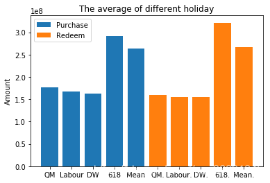
# 画出节假日与平时的均值fig = plt.figure()
index_list = ['QM','Labour','DW','618','Mean']
label_list = [np.mean(qingming['total_purchase_amt']), np.mean(labour['total_purchase_amt']),np.mean(duanwu['total_purchase_amt']),np.mean(data618['total_purchase_amt']),np.mean(total_balance_1['total_purchase_amt'])]
plt.bar(index_list, label_list, label="Purchase")index_list = ['QM.','Labour.','DW.','618.','Mean.']
label_list = [np.mean(qingming['total_redeem_amt']), np.mean(labour['total_redeem_amt']),np.mean(duanwu['total_redeem_amt']),np.mean(data618['total_redeem_amt']),np.mean(total_balance_1['total_redeem_amt'])]
plt.bar(index_list, label_list, label="Redeem")
plt.title("The average of different holiday")
plt.ylabel("Amount")
plt.legend()
plt.show()
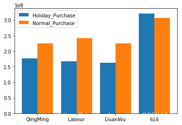
# 画出节假日购买量与其所处翌日的对比import numpy as np
import matplotlib.pyplot as plt
size = 4
x = np.arange(size)total_width, n = 0.8, 2
width = total_width / n
x = x - (total_width - width) / 2a = [176250006, 167825284, 162844282,321591063]
b = [225337516, 241859315, 225337516,307635449]plt.bar(x, a,  width=width, label='Holiday_Purchase')
plt.bar(x + width, b, width=width, label='Normal_Purchase')
plt.xticks(x + width / 2, ('QingMing', 'Labour', 'DuanWu', '618'))
plt.legend()
plt.show()
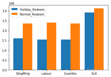
# 画出节假日赎回量与其所处翌日的对比import numpy as np
import matplotlib.pyplot as plt
size = 4
x = np.arange(size)total_width, n = 0.8, 2
width = total_width / n
x = x - (total_width - width) / 2a = [159914308, 154717620, 154366940,291016763]
b = [235439685, 240364238, 235439685,313310347]plt.bar(x, a,  width=width, label='Holiday_Redeem')
plt.bar(x + width, b, width=width, label='Normal_Redeem')
plt.xticks(x + width / 2, ('QingMing', 'Labour', 'DuanWu', '618'))
plt.legend()
plt.show()
六、对于节假日周边日期的分析
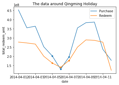
# 画出清明节与周边日期的时序图qingming_around = total_balance[(total_balance['date'] >= datetime.date(2014,4,1)) & (total_balance['date'] < datetime.date(2014,4,13))]
ax = sns.lineplot(x="date", y="total_purchase_amt", data=qingming_around, label='Purchase')
ax = sns.lineplot(x="date", y="total_redeem_amt", data=qingming_around, label='Redeem', ax=ax)
ax = sns.scatterplot(x="date", y="total_purchase_amt", data=qingming, ax=ax)
ax = sns.scatterplot(x="date", y="total_redeem_amt", data=qingming, ax=ax)
plt.title("The data around Qingming Holiday")
ax.legend()
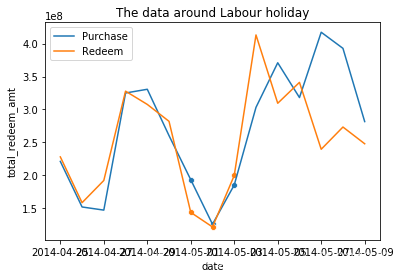
# 画出劳动节与周边日期的时序图labour_around = total_balance[(total_balance['date'] >= datetime.date(2014,4,25)) & (total_balance['date'] < datetime.date(2014,5,10))]
ax = sns.lineplot(x="date", y="total_purchase_amt", data=labour_around, label='Purchase')
ax = sns.lineplot(x="date", y="total_redeem_amt", data=labour_around, label='Redeem', ax=ax)
ax = sns.scatterplot(x="date", y="total_purchase_amt", data=labour, ax=ax)
ax = sns.scatterplot(x="date", y="total_redeem_amt", data=labour, ax=ax)
plt.title("The data around Labour holiday")
ax.legend()
# # 画出端午节与周边日期的时序图duanwu_around = total_balance[(total_balance['date'] >= datetime.date(2014,5,25)) & (total_balance['date'] < datetime.date(2014,6,7))]
ax = sns.lineplot(x="date", y="total_purchase_amt", data=duanwu_around, label='Purchase')
ax = sns.lineplot(x="date", y="total_redeem_amt", data=duanwu_around, label='Redeem', ax=ax)
ax = sns.scatterplot(x="date", y="total_purchase_amt", data=duanwu, ax=ax)
ax = sns.scatterplot(x="date", y="total_redeem_amt", data=duanwu, ax=ax)
plt.title("The data around Duanwu Holiday")
ax.legend()
# 画出中秋与周边日期的时序图zhongqiu = total_balance[(total_balance['date'] >= datetime.date(2013,9,19)) & (total_balance['date'] < datetime.date(2013,9,22))]
zhongqiu_around = total_balance[(total_balance['date'] >= datetime.date(2013,9,14)) & (total_balance['date'] < datetime.date(2013,9,28))]
ax = sns.lineplot(x="date", y="total_purchase_amt", data=zhongqiu_around, label='Purchase')
ax = sns.lineplot(x="date", y="total_redeem_amt", data=zhongqiu_around, label='Redeem', ax=ax)
ax = sns.scatterplot(x="date", y="total_purchase_amt", data=zhongqiu, ax=ax)
ax = sns.scatterplot(x="date", y="total_redeem_amt", data=zhongqiu, ax=ax)
plt.title("The data around MiddleAutumn Holiday(in 2013)")
ax.legend()
七、对于异常值的分析
# 画出用户交易纪录的箱型图sns.boxplot(data_balance['total_purchase_amt'])
plt.title("The abnormal value of total purchase")
Text(0.5, 1.0, 'The abnormal value of total purchase')

# 对于购买2e8的用户的交易行为分析data_balance[data_balance['user_id'] == 14592].sort_values(by = 'total_redeem_amt',axis = 0,ascending = False).head()
user_id	report_date	tBalance	yBalance	total_purchase_amt	direct_purchase_amt	purchase_bal_amt	purchase_bank_amt	total_redeem_amt	consume_amt	...	category1	category2	category3	category4	date	day	month	year	week	weekday
1453311	14592	20131104	99457728	0	201768328	201768328	201275171	493157	102310600	0	...	NaN	NaN	NaN	NaN	2013-11-04	4	11	2013	45	0
1453388	14592	20140616	0	98964529	1966014	1953569	0	1953569	100930543	0	...	NaN	NaN	NaN	NaN	2014-06-16	16	6	2014	25	0
1453227	14592	20131226	367063	98296082	17369	0	0	0	97946388	0	...	NaN	NaN	NaN	NaN	2013-12-26	26	12	2013	52	3
1453313	14592	20131105	97458675	99457728	4899446	4899446	4899446	0	6898499	0	...	NaN	NaN	NaN	NaN	2013-11-05	5	11	2013	45	1
1453355	14592	20140617	0	0	339679	339679	0	339679	339679	0	...	NaN	NaN	NaN	NaN	2014-06-17	17	6	2014	25	1
5 rows × 24 columns1311 Bought 2E Seal 1E
1312        Seal 1E
1405 Bought 0.9E
1406        Seal 1E
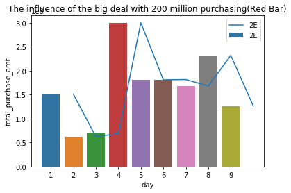
# 画出单笔交易为2e8的那天的总交易量及附近几天的交易量e2 = total_balance[(total_balance['date'] >= datetime.date(2013,11,1)) & (total_balance['date'] < datetime.date(2013,11,10))]
ax = sns.barplot(x="day", y="total_purchase_amt", data=e2, label='2E')
ax = sns.lineplot(x="day", y="total_purchase_amt", data=e2, label='2E')
plt.title("The influence of the big deal with 200 million purchasing(Red Bar)")
ax.legend()
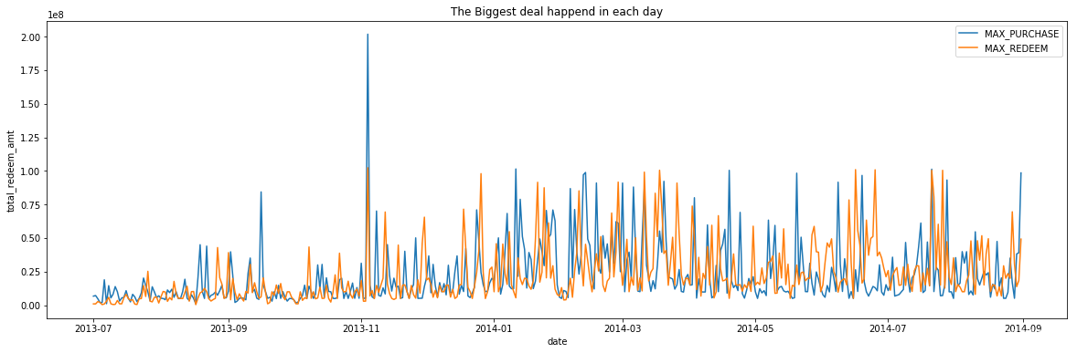
# 画出每日单笔最大交易的时序图plt.figure(figsize=(20, 6))
ax = sns.lineplot(x="date", y="total_purchase_amt", data=data_balance[['total_purchase_amt', 'date']].groupby('date', as_index=False).max(), label='MAX_PURCHASE')
ax = sns.lineplot(x="date", y="total_redeem_amt", data=data_balance[['total_redeem_amt', 'date']].groupby('date', as_index=False).max(), label='MAX_REDEEM')
plt.title("The Biggest deal happend in each day")
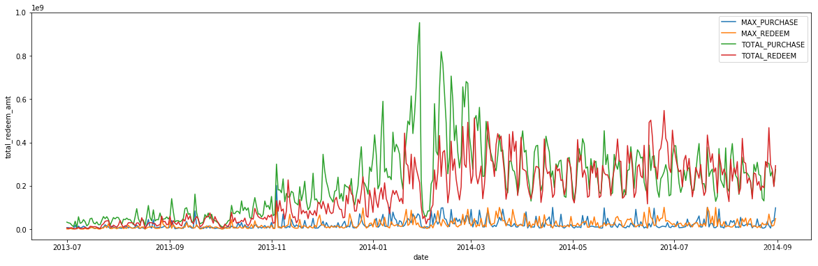
# 画出每日单笔最大交易以及总交易额的时序图plt.figure(figsize=(20, 6))
ax = sns.lineplot(x="date", y="total_purchase_amt", data=data_balance[['total_purchase_amt', 'date']].groupby('date', as_index=False).max(), label='MAX_PURCHASE')
ax = sns.lineplot(x="date", y="total_redeem_amt", data=data_balance[['total_redeem_amt', 'date']].groupby('date', as_index=False).max(), label='MAX_REDEEM')
ax = sns.lineplot(x="date", y="total_purchase_amt", data=data_balance[['total_purchase_amt', 'date']].groupby('date', as_index=False).sum(), label='TOTAL_PURCHASE')
ax = sns.lineplot(x="date", y="total_redeem_amt", data=data_balance[['total_redeem_amt', 'date']].groupby('date', as_index=False).sum(), label='TOTAL_REDEEM')
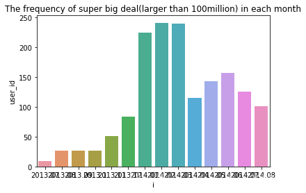
# 画出每个月大额交易的频次直方图big_frequancy = data_balance[(data_balance['total_purchase_amt'] > 10000000) | (data_balance['total_redeem_amt'] > 10000000)][['month','year','user_id']].groupby(['year','month'], as_index=False).count()
big_frequancy['i'] = big_frequancy['year']  + big_frequancy['month'] / 100
ax = sns.barplot(x="i", y="user_id", data=big_frequancy)
plt.title("The frequency of super big deal(larger than 100million) in each month")
# 获取大额交易的数据集data_balance['big_purchase'] = 0
data_balance.loc[data_balance['total_purchase_amt'] > 1000000, 'big_purchase'] = 1
data_balance['big_redeem'] = 0
data_balance.loc[data_balance['total_redeem_amt'] > 1000000, 'big_redeem'] = 1# 对大额交易按每天做聚合操作big_purchase = data_balance[data_balance['big_purchase'] == 1].groupby(['date'], as_index=False)['total_purchase_amt'].sum()
small_purchase = data_balance[data_balance['big_purchase'] == 0].groupby(['date'], as_index=False)['total_purchase_amt'].sum()
big_redeem = data_balance[data_balance['big_redeem'] == 1].groupby(['date'], as_index=False)['total_redeem_amt'].sum()
small_redeem = data_balance[data_balance['big_redeem'] == 0].groupby(['date'], as_index=False)['total_redeem_amt'].sum()# 画出大额交易与小额交易的时序分布图fig = plt.figure(figsize=(20,6))
plt.plot(big_purchase['date'], big_purchase['total_purchase_amt'],label='big_purchase')
plt.plot(big_redeem['date'], big_redeem['total_redeem_amt'],label='big_redeem')plt.plot(small_purchase['date'], small_purchase['total_purchase_amt'],label='small_purchase')
plt.plot(small_redeem['date'], small_redeem['total_redeem_amt'],label='small_redeem')
plt.legend(loc='best')
plt.title("The time series of big deal of Purchase and Redeem from July.13 to Sep.14")
plt.xlabel("Time")
plt.ylabel("Amount")
plt.show()

# 画出大额交易与小额交易的分布估计图plt.figure(figsize=(12,10))plt.subplot(2,2,1)
for i in range(4, 9):sns.kdeplot(big_purchase[(big_purchase['date'] >= datetime.date(2014,i,1)) & (big_purchase['date'] < datetime.date(2014,i+1,1))]['total_purchase_amt'],label='14Y,'+str(i)+'M')
plt.title('BIG PURCHASE')plt.subplot(2,2,2)
for i in range(4, 9):sns.kdeplot(small_purchase[(small_purchase['date'] >= datetime.date(2014,i,1)) & (small_purchase['date'] < datetime.date(2014,i+1,1))]['total_purchase_amt'],label='14Y,'+str(i)+'M')
plt.title('SMALL PURCHASE')plt.subplot(2,2,3)
for i in range(4, 9):sns.kdeplot(big_redeem[(big_redeem['date'] >= datetime.date(2014,i,1)) & (big_redeem['date'] < datetime.date(2014,i+1,1))]['total_redeem_amt'],label='14Y,'+str(i)+'M')
plt.title('BIG REDEEM')plt.subplot(2,2,4)
for i in range(4, 9):sns.kdeplot(small_redeem[(small_redeem['date'] >= datetime.date(2014,i,1)) & (small_redeem['date'] < datetime.date(2014,i+1,1))]['total_redeem_amt'],label='14Y,'+str(i)+'M')
plt.title('SMALL REDEEM')

# 添加时间戳big_purchase['weekday'] = big_purchase['date'].dt.weekday
small_purchase['weekday'] = small_purchase['date'].dt.weekday
big_redeem['weekday'] = big_redeem['date'].dt.weekday
small_redeem['weekday'] = small_redeem['date'].dt.weekday
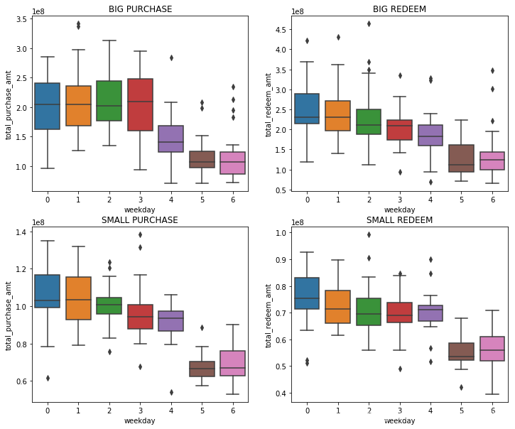
# 分析大额小额的翌日分布plt.figure(figsize=(12, 10))ax = plt.subplot(2,2,1)
ax = sns.boxplot(x="weekday", y="total_purchase_amt", data=big_purchase[big_purchase['date'] >= datetime.date(2014,4,1)])
plt.title('BIG PURCHASE')ax = plt.subplot(2,2,2)
ax = sns.boxplot(x="weekday", y="total_redeem_amt", data=big_redeem[big_redeem['date'] >= datetime.date(2014,4,1)])
plt.title('BIG REDEEM')ax = plt.subplot(2,2,3)
ax = sns.boxplot(x="weekday", y="total_purchase_amt", data=small_purchase[small_purchase['date'] >= datetime.date(2014,4,1)])
plt.title('SMALL PURCHASE')ax = plt.subplot(2,2,4)
ax = sns.boxplot(x="weekday", y="total_redeem_amt", data=small_redeem[small_redeem['date'] >= datetime.date(2014,4,1)])
plt.title('SMALL REDEEM')
八、分析用户交易纪录表中其他变量
# 截断数据集data_balance_1 = data_balance[data_balance['date'] > datetime.datetime(2014,4,1)]# 画出用户交易纪录表中其他变量与标签的相关性图feature = ['total_purchase_amt','total_redeem_amt', 'report_date', 'tBalance', 'yBalance', 'direct_purchase_amt', 'purchase_bal_amt', 'purchase_bank_amt','consume_amt', 'transfer_amt', 'tftobal_amt','tftocard_amt', 'share_amt']sns.heatmap(data_balance_1[feature].corr(), linewidths = 0.05)
plt.title("The coleration between each feature in User_Balance_Table")

九、对于银行及支付宝利率的分析
# 读取银行利率并添加时间戳bank = pd.read_csv(dataset_path + "mfd_bank_shibor.csv")
bank = bank.rename(columns = {'mfd_date': 'date'})
bank_features = [x for x in bank.columns if x not in ['date']]
bank['date'] = pd.to_datetime(bank['date'], format= "%Y%m%d")
bank['day'] = bank['date'].dt.day
bank['month'] = bank['date'].dt.month
bank['year'] = bank['date'].dt.year
bank['week'] = bank['date'].dt.week
bank['weekday'] = bank['date'].dt.weekday
# 读取支付宝利率并添加时间戳share = pd.read_csv(dataset_path + 'mfd_day_share_interest.csv')
share = share.rename(columns = {'mfd_date': 'date'})
share_features = [x for x in share.columns if x not in ['date']]
share['date'] = pd.to_datetime(share['date'], format= "%Y%m%d")
share['day'] = share['date'].dt.day
share['month'] = share['date'].dt.month
share['year'] = share['date'].dt.year
share['week'] = share['date'].dt.week
share['weekday'] = share['date'].dt.weekday
# 画出上一天银行及支付宝利率与标签的相关性图bank['last_date'] = bank['date'] + datetime.timedelta(days=1)
plt.figure(figsize=(12,4))
plt.subplot(1,3,1)
plt.title("The coleration between each lastday bank rate and total purchase")
temp = pd.merge(bank[['last_date']+bank_features], total_balance, left_on='last_date', right_on='date')[['total_purchase_amt']+bank_features]
sns.heatmap(temp.corr(), linewidths = 0.05)
plt.subplot(1,3,3)
plt.title("The coleration between each lastday bank rate and total redeem")
temp = pd.merge(bank[['last_date']+bank_features], total_balance, left_on='last_date', right_on='date')[['total_redeem_amt']+bank_features]
sns.heatmap(temp.corr(), linewidths = 0.05)

# 画出上一星期银行及支付宝利率与标签的相关性图bank['last_week'] = bank['week'] + 1
plt.figure(figsize=(12,4))
plt.subplot(1,3,1)
plt.title("The coleration between each last week bank rate and total purchase")
temp = pd.merge(bank[['last_week','weekday']+bank_features], total_balance, left_on=['last_week','weekday'], right_on=['week','weekday'])[['total_purchase_amt']+bank_features]
sns.heatmap(temp.corr(), linewidths = 0.05)
plt.subplot(1,3,3)
plt.title("The coleration between each last week bank rate and total redeem")
temp = pd.merge(bank[['last_week','weekday']+bank_features], total_balance, left_on=['last_week','weekday'], right_on=['week','weekday'])[['total_redeem_amt']+bank_features]
sns.heatmap(temp.corr(), linewidths = 0.05)

# 分别画出上一星期银行及支付宝利率与大额小额数据的相关性图bank['last_date'] = bank['date'] + datetime.timedelta(days=1)
plt.figure(figsize=(12,4))
plt.subplot(1,3,1)
plt.title("The coleration of Small Rate purchase")
temp = pd.merge(bank[['last_date']+bank_features], small_purchase, left_on='last_date', right_on='date')[['total_purchase_amt']+bank_features]
sns.heatmap(temp.corr(), linewidths = 0.05)
plt.subplot(1,3,3)
plt.title("The coleration of Small Rate redeem")
temp = pd.merge(bank[['last_date']+bank_features], small_redeem, left_on='last_date', right_on='date')[['total_redeem_amt']+bank_features]
sns.heatmap(temp.corr(), linewidths = 0.05)  bank['last_date'] = bank['date'] + datetime.timedelta(days=1)
plt.figure(figsize=(12,4))
plt.subplot(1,3,1)
plt.title("The coleration of Big Rate purchase")
temp = pd.merge(bank[['last_date']+bank_features], big_purchase, left_on='last_date', right_on='date')[['total_purchase_amt']+bank_features]
sns.heatmap(temp.corr(), linewidths = 0.05)
plt.subplot(1,3,3)
plt.title("The coleration of Big Rate redeem")
temp = pd.merge(bank[['last_date']+bank_features], big_redeem, left_on='last_date', right_on='date')[['total_redeem_amt']+bank_features]
sns.heatmap(temp.corr(), linewidths = 0.05)


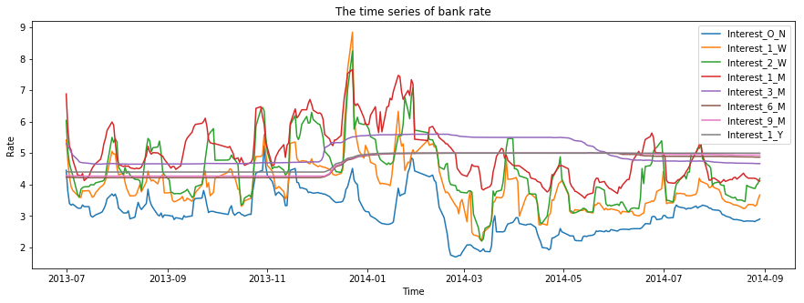
# 画出银行利率的时序图plt.figure(figsize=(15,5))
for i in bank_features:plt.plot(bank['date'], bank[[i]] ,label=i)
plt.legend()
plt.title("The time series of bank rate")
plt.xlabel("Time")
plt.ylabel("Rate")
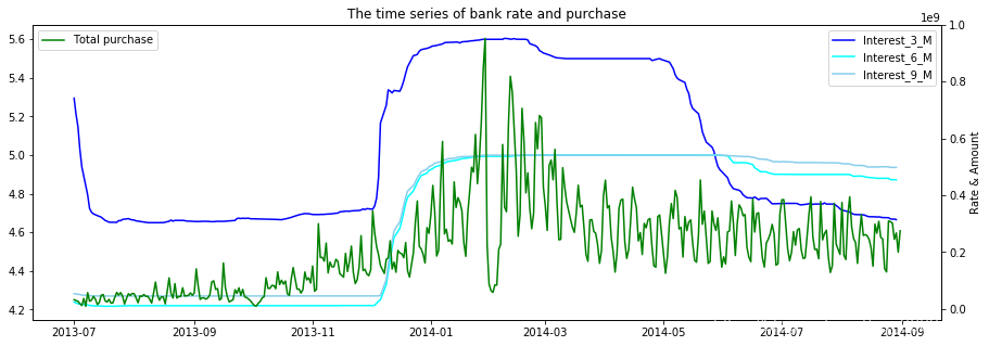
# 画出部分银行利率与购买量的时序图fig,ax1 = plt.subplots(figsize=(15,5))
plt.plot(bank['date'], bank['Interest_3_M'],'b',label="Interest_3_M")
plt.plot(bank['date'], bank['Interest_6_M'],'cyan',label="Interest_6_M")
plt.plot(bank['date'], bank['Interest_9_M'],'skyblue',label="Interest_9_M")plt.legend()ax2=ax1.twinx()
plt.plot(total_balance['date'], total_balance['total_purchase_amt'],'g',label="Total purchase")plt.legend(loc=2)
plt.title("The time series of bank rate and purchase")
plt.xlabel("Time")
plt.ylabel("Rate & Amount")
plt.show()
# 画出部分银行利率与赎回量的时序图fig,ax1 = plt.subplots(figsize=(15,5))
plt.plot(bank['date'], bank['Interest_3_M'],'b',label="Interest_3_M")
plt.plot(bank['date'], bank['Interest_6_M'],'cyan',label="Interest_6_M")
plt.plot(bank['date'], bank['Interest_9_M'],'skyblue',label="Interest_9_M")plt.legend()ax2=ax1.twinx()
plt.plot(total_balance['date'], total_balance['total_redeem_amt'],'g',label="Total redeem")plt.legend(loc=2)
plt.title("The time series of bank rate and redeem")
plt.xlabel("Time")
plt.ylabel("Rate & Amount")plt.show()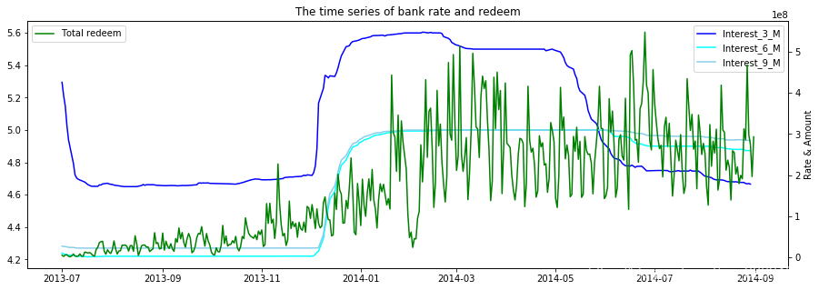
The information for Share rate
# 画出支付宝利率与标签的相关性图share['last_date'] = share['date'] + datetime.timedelta(days=1)
plt.figure(figsize=(12,4))
plt.subplot(1,3,1)
temp = pd.merge(share[['last_date']+share_features], total_balance, left_on='last_date', right_on='date')[['total_purchase_amt']+share_features]
sns.heatmap(temp.corr(), linewidths = 0.05, vmin = 0)
plt.subplot(1,3,3)
temp = pd.merge(share[['last_date']+share_features], total_balance, left_on='last_date', right_on='date')[['total_redeem_amt']+share_features]
sns.heatmap(temp.corr(), linewidths = 0.05, vmin = 0)

# 画出银行利率与标签的相关性图share['last_week'] = share['week'] + 1
plt.figure(figsize=(12,4))
plt.subplot(1,3,1)
temp = pd.merge(share[['last_week','weekday']+share_features], total_balance, left_on=['last_week','weekday'], right_on=['week','weekday'])[['total_purchase_amt']+share_features]
sns.heatmap(temp.corr(), linewidths = 0.05, vmin = 0)
plt.subplot(1,3,3)
temp = pd.merge(share[['last_week','weekday']+share_features], total_balance, left_on=['last_week','weekday'], right_on=['week','weekday'])[['total_redeem_amt']+share_features]
sns.heatmap(temp.corr(), linewidths = 0.05, vmin = 0)

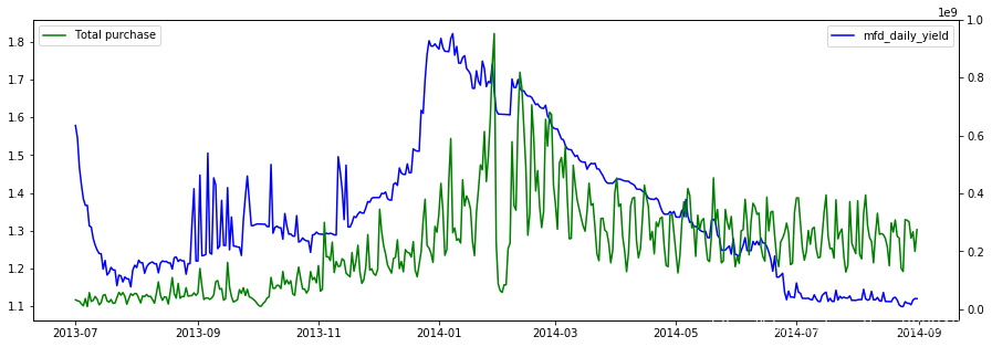
# 画出支付宝利率与购买量的时序图fig,ax1 = plt.subplots(figsize=(15,5))
for i in share_features:plt.plot(share['date'], share[i],'b',label=i)break
plt.legend()
ax2=ax1.twinx()
plt.plot(total_balance['date'], total_balance['total_purchase_amt'],'g',label="Total purchase")
plt.legend(loc=2)
plt.show()
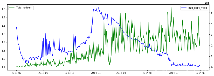
# 画出支付宝利率与赎回量的时序图fig,ax1 = plt.subplots(figsize=(15,5))
for i in share_features:plt.plot(share['date'], share[i],'b',label=i)break
plt.legend()
ax2=ax1.twinx()
plt.plot(total_balance['date'], total_balance['total_redeem_amt'],'g',label="Total redeem")
plt.legend(loc=2)
plt.show()
# 画出大额小额数据与支付宝利率的相关性图share['last_date'] = share['date'] + datetime.timedelta(days=1)
plt.figure(figsize=(12,4))
plt.subplot(1,3,1)
temp = pd.merge(share[['last_date']+share_features], small_purchase, left_on='last_date', right_on='date')[['total_purchase_amt']+share_features]
sns.heatmap(temp.corr(), linewidths = 0.05, vmin=0)
plt.title("SMALL PURCHASE")
plt.subplot(1,3,3)
plt.title("SMALL REDEEM")
temp = pd.merge(share[['last_date']+share_features], small_redeem, left_on='last_date', right_on='date')[['total_redeem_amt']+share_features]
sns.heatmap(temp.corr(), linewidths = 0.05, vmin=0)  share['last_date'] = share['date'] + datetime.timedelta(days=1)
plt.figure(figsize=(12,4))
plt.subplot(1,3,1)
plt.title("BIG PURCHASE")
temp = pd.merge(share[['last_date']+share_features], big_purchase, left_on='last_date', right_on='date')[['total_purchase_amt']+share_features]
sns.heatmap(temp.corr(), linewidths = 0.05, vmin=0)
plt.subplot(1,3,3)
plt.title("BIG REDEEM")
temp = pd.merge(share[['last_date']+share_features], big_redeem, left_on='last_date', right_on='date')[['total_redeem_amt']+share_features]
sns.heatmap(temp.corr(), linewidths = 0.05, vmin=0)


# 画出银行利率与支付宝利率的时序图fig,ax1 = plt.subplots(figsize=(15,5))
plt.plot(bank['date'], bank['Interest_3_M'],c='g',label= 'BANK')plt.legend()
ax2=ax1.twinx()
plt.plot(share['date'], share['mfd_daily_yield'],label='SHARE')
plt.legend(loc=2)
plt.show()
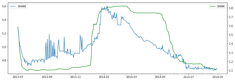
It seems that:
- The influence of share is more likely to act on Purchase
- The influence of bank rate is more likely to act on Redeem
- The influence of share rate is for short
- The influence of bank rate is for long
based on above analysis, we can simply find three features:
-
the weekday
-
is it weekend
-
is it holidy
-
the distance from the start of week(monday)
-
the distance from the end of week(sunday)
-
the distance from the holiday centre(centre of QingMing DuanWu
Labour ZhongQiu) -
the distance from the start of month
-
the distance from the end of month
-
the mean/max/min value of the same week in last month
-
the value in last day of last month