KMenas算法
#导入KMeans模块
from sklearn.cluster import KMeans
from sklearn.datasets import make_blobs
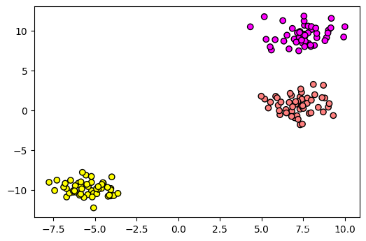
#随机生成含150个类别数为3的数据集
X,y=make_blobs(n_samples=150,centers=3,random_state=8)
#数据可视化
import matplotlib.pyplot as plt
%matplotlib inline
plt.figure(dpi=100)
plt.scatter(X[:,0],X[:,1],c=y,cmap=plt.cm.spring,edgecolors='k')
<matplotlib.collections.PathCollection at 0x24dbd2a2dd8>
#模块实例化
kmeans=KMeans(n_clusters=3)
#模型训练
kmeans.fit(X)
KMeans(algorithm='auto', copy_x=True, init='k-means++', max_iter=300,n_clusters=3, n_init=10, n_jobs=None, precompute_distances='auto',random_state=None, tol=0.0001, verbose=0)
import numpy as np
from matplotlib.colors import ListedColormap
#定义图像中分区的颜色和散点的颜色
cmap_light = ListedColormap(['#FFAAAA', '#AAFFAA', '#AAAAFF'])
cmap_bold = ListedColormap(['#FF0000', '#00FF00', '#0000FF'])
#分别用样本的两个特征值创建图像的横轴和纵轴
x_min, x_max = X[:, 0].min() - 1, X[:, 0].max() + 1
y_min, y_max = X[:, 1].min() - 1, X[:, 1].max() + 1
xx, yy = np.meshgrid(np.arange(x_min, x_max, .02),np.arange(y_min, y_max, .02))
Z = kmeans.predict(np.c_[xx.ravel(), yy.ravel()])
#给每个分类中的样本分配不同的颜色
Z = Z.reshape(xx.shape)
plt.pcolormesh(xx, yy, Z, cmap=cmap_light)
#用散点把样本表示出来
plt.scatter(X[:, 0], X[:, 1], c=y, cmap = plt.cm.spring, edgecolor='k', s=20)
plt.xlim(xx.min(), xx.max())
plt.ylim(yy.min(), yy.max())
plt.title("K-Means Cluster")

Text(0.5, 1.0, 'K-Means Cluster')
#查看聚类中心点的坐标
kmeans.cluster_centers_
array([[ 7.51338019, 9.44881625],[-5.43790266, -9.83963795],[ 7.21711781, 0.68887741]])
#将数据中心点可视化
import numpy as np
from matplotlib.colors import ListedColormap
#定义图像中分区的颜色和散点的颜色
cmap_light = ListedColormap(['#FFAAAA', '#AAFFAA', '#AAAAFF'])
cmap_bold = ListedColormap(['#FF0000', '#00FF00', '#0000FF'])
#分别用样本的两个特征值创建图像的横轴和纵轴
x_min, x_max = X[:, 0].min() - 1, X[:, 0].max() + 1
y_min, y_max = X[:, 1].min() - 1, X[:, 1].max() + 1
xx, yy = np.meshgrid(np.arange(x_min, x_max, .02),np.arange(y_min, y_max, .02))
Z = kmeans.predict(np.c_[xx.ravel(), yy.ravel()])
#给每个分类中的样本分配不同的颜色
Z = Z.reshape(xx.shape)
plt.pcolormesh(xx, yy, Z, cmap=cmap_light)
#用散点把样本表示出来
plt.scatter(X[:, 0], X[:, 1], c=y, cmap = plt.cm.spring, edgecolor='k', s=20)
plt.scatter(kmeans.cluster_centers_[:,0],kmeans.cluster_centers_[:,1],s=200,marker='*',c='red',label='centroids')
plt.legend()
plt.xlim(xx.min(), xx.max())
plt.ylim(yy.min(), yy.max())
plt.title("K-Means Cluster")

Text(0.5, 1.0, 'K-Means Cluster')
[外链图片转存失败,源站可能有防盗链机制,建议将图片保存下来直接上传(img-vki9Yroa-1645627108907)(output_7_2.png)]
#查看数据标签
kmeans.labels_
array([0, 2, 1, 0, 1, 1, 2, 1, 2, 1, 1, 2, 0, 0, 2, 2, 2, 2, 0, 2, 0, 0,2, 0, 1, 2, 0, 1, 1, 1, 0, 1, 2, 2, 0, 2, 0, 1, 1, 2, 2, 1, 1, 1,2, 2, 0, 0, 0, 1, 2, 2, 1, 1, 0, 2, 1, 2, 1, 0, 0, 2, 2, 0, 0, 2,0, 2, 2, 0, 0, 0, 0, 1, 0, 2, 2, 1, 0, 0, 0, 1, 1, 1, 2, 2, 1, 0,1, 2, 2, 1, 1, 2, 0, 1, 0, 1, 2, 2, 0, 0, 0, 2, 1, 1, 2, 1, 0, 2,1, 0, 0, 1, 2, 0, 1, 2, 2, 1, 1, 1, 1, 0, 0, 0, 1, 2, 2, 2, 0, 1,0, 1, 2, 0, 0, 0, 0, 0, 0, 1, 2, 1, 1, 2, 2, 1, 1, 2])
#查看运行时迭代的次数
kmeans.n_iter_
2
#查看各样本与其最近的类中心的距离之和,簇内误差平方和
kmeans.inertia_
329.18213511898057
#肘方法,确定k值
distortion=[]
for i in range(1,20):km=KMeans(n_clusters=i,init='k-means++',random_state=8)km.fit(X)distortion.append(km.inertia_)
plt.plot(range(1, 20), distortion, marker='o')
plt.xticks(range(1, 20))
plt.grid(linestyle='--')
plt.xlabel('Number of clusters')
plt.ylabel('Distortion')
Text(0, 0.5, 'Distortion')

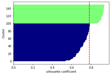
#计算并绘制轮廓系数
km=KMeans(n_clusters=2)
y_km=km.fit_predict(X)
from matplotlib import cm
from sklearn.metrics import silhouette_samples
cluster_labels=np.unique(y_km)
n_clusters=cluster_labels.shape[0]
silhouette_vals=silhouette_samples(X,y_km,metric='euclidean')
y_ax_lower,y_ax_upper= 0,0
yticks = []
for i ,c in enumerate(cluster_labels):c_silhouette_vals = silhouette_vals[y_km == c]c_silhouette_vals.sort()y_ax_upper += len(c_silhouette_vals)color = cm. jet(i/n_clusters)plt.barh(range(y_ax_lower, y_ax_upper),c_silhouette_vals,height=1.0,edgecolor='none',color=color)yticks.append((y_ax_lower+y_ax_upper)/2)y_ax_lower += len(c_silhouette_vals)silhouette_avg = np.mean(silhouette_vals)plt.axvline(silhouette_avg,color='red',linestyle='--')
plt.ylabel("Cluster")
plt.xlabel("silhouette coefficient")
Text(0.5, 0, 'silhouette coefficient')
DBSCAN算法
from sklearn.cluster import DBSCAN
#生成模拟数据集
from sklearn.datasets import make_moons
X,y=make_moons(n_samples=200,noise=0.05,random_state=8)
#数据可视化
plt.scatter(X[:,0],X[:,1],c=y,cmap=plt.cm.spring,edgecolors='k')
<matplotlib.collections.PathCollection at 0x24dfc0ddd68>

#利用K-Means算法聚类
#模型实例化
kmeans=KMeans(n_clusters=2,init='random')
#模型训练与预测
y_km=kmeans.fit_predict(X)
#将数据中心点可视化
import numpy as np
from matplotlib.colors import ListedColormap
#定义图像中分区的颜色和散点的颜色
cmap_light = ListedColormap(['#FFAAAA', '#AAFFAA', '#AAAAFF'])
cmap_bold = ListedColormap(['#FF0000', '#00FF00', '#0000FF'])
#分别用样本的两个特征值创建图像的横轴和纵轴
x_min, x_max = X[:, 0].min() - 1, X[:, 0].max() + 1
y_min, y_max = X[:, 1].min() - 1, X[:, 1].max() + 1
xx, yy = np.meshgrid(np.arange(x_min, x_max, .02),np.arange(y_min, y_max, .02))
Z = kmeans.predict(np.c_[xx.ravel(), yy.ravel()])
#给每个分类中的样本分配不同的颜色
Z = Z.reshape(xx.shape)
plt.pcolormesh(xx, yy, Z, cmap=cmap_light)
#用散点把样本表示出来
plt.scatter(X[:, 0], X[:, 1], c=y, cmap = plt.cm.spring, edgecolor='k', s=20)
plt.scatter(kmeans.cluster_centers_[:,0],kmeans.cluster_centers_[:,1],s=200,marker='*',c='red',label='centroids')
plt.legend()
plt.grid()
plt.xlim(xx.min(), xx.max())
plt.ylim(yy.min(), yy.max())
plt.title("K-Means Cluster")

Text(0.5, 1.0, 'K-Means Cluster')
#结果可视化
plt.scatter(X[y_km==0,0],X[y_km==0,1],c='red',marker='o',s=40,label='cluster 1',edgecolor='k')
plt.scatter(X[y_km==1,0],X[y_km==1,1],c='green',marker='s',s=40,label='cluster 2',edgecolor='k')
plt.title('K-means clustering')
plt.legend()
<matplotlib.legend.Legend at 0x24dfc0a1c88>
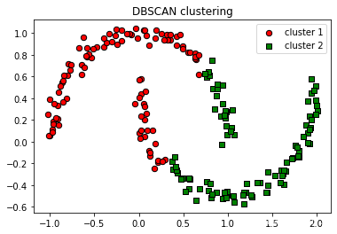
#利用DBSCAN聚类
#导入DBSCAN模块
from sklearn.cluster import DBSCAN
#模型实例化
db=DBSCAN(eps=0.2,min_samples=5)
#训练模型并预测
y_db=db.fit_predict(X)
#DBSCAN结果可视化
plt.scatter(X[y_km==0,0],X[y_km==0,1],c='red',marker='o',s=40,label='cluster 1',edgecolor='k')
plt.scatter(X[y_km==1,0],X[y_km==1,1],c='green',marker='s',s=40,label='cluster 2',edgecolor='k')
plt.title('DBSCAN clustering')
plt.legend()
<matplotlib.legend.Legend at 0x24dfc5b6320>
!
%matplotlib inline
import pandas as pd
import matplotlib.pyplot as plt
dbscan_data=pd.read_csv(r'C:\Users\86139\Desktop\dbscan_data.txt')
dbscan_data.head()
plt.scatter(dbscan_data['x1'],dbscan_data['x2'])
<matplotlib.collections.PathCollection at 0x24dfe0f40b8>

import numpy as np
from sklearn.cluster import DBSCAN
db=DBSCAN(eps=0.1,min_samples=10)
db.fit(dbscan_data)
DBSCAN(algorithm='auto', eps=0.1, leaf_size=30, metric='euclidean',metric_params=None, min_samples=10, n_jobs=None, p=None)
db.labels_
array([0, 0, 0, ..., 2, 1, 1], dtype=int64)
labels6=db.labels_
dbscan_data['cluster_db']=labels6
colors=np.array(['red','green','blue','yellow','teal','orange','cyan','black','goldenrod','tomato'])
plt.figure(figsize=(10,8))
plt.scatter(dbscan_data['x1'],dbscan_data['x2'],c=colors[dbscan_data['cluster_db']])
<matplotlib.collections.PathCollection at 0x24dfe148400>

层次聚类
seeds_df=pd.read_csv(r'C:\Users\86139\Desktop\seeds-less-rows.csv')
seeds_df.head()
| area | perimeter | compactness | length | width | asymmetry_coefficient | groove_length | grain_variety | |
|---|---|---|---|---|---|---|---|---|
| 0 | 14.88 | 14.57 | 0.8811 | 5.554 | 3.333 | 1.018 | 4.956 | Kama wheat |
| 1 | 14.69 | 14.49 | 0.8799 | 5.563 | 3.259 | 3.586 | 5.219 | Kama wheat |
| 2 | 14.03 | 14.16 | 0.8796 | 5.438 | 3.201 | 1.717 | 5.001 | Kama wheat |
| 3 | 13.99 | 13.83 | 0.9183 | 5.119 | 3.383 | 5.234 | 4.781 | Kama wheat |
| 4 | 14.11 | 14.26 | 0.8722 | 5.520 | 3.168 | 2.688 | 5.219 | Kama wheat |
seeds_df.grain_variety.value_counts()
Kama wheat        14
Rosa wheat        14
Canadian wheat    14
Name: grain_variety, dtype: int64
varieties=list(seeds_df.pop('grain_variety'))
samples=seeds_df.values
samples
array([[14.88 , 14.57 , 0.8811, 5.554 , 3.333 , 1.018 , 4.956 ],[14.69 , 14.49 , 0.8799, 5.563 , 3.259 , 3.586 , 5.219 ],[14.03 , 14.16 , 0.8796, 5.438 , 3.201 , 1.717 , 5.001 ],[13.99 , 13.83 , 0.9183, 5.119 , 3.383 , 5.234 , 4.781 ],[14.11 , 14.26 , 0.8722, 5.52 , 3.168 , 2.688 , 5.219 ],[13.02 , 13.76 , 0.8641, 5.395 , 3.026 , 3.373 , 4.825 ],[15.49 , 14.94 , 0.8724, 5.757 , 3.371 , 3.412 , 5.228 ],[16.2 , 15.27 , 0.8734, 5.826 , 3.464 , 2.823 , 5.527 ],[13.5 , 13.85 , 0.8852, 5.351 , 3.158 , 2.249 , 5.176 ],[15.36 , 14.76 , 0.8861, 5.701 , 3.393 , 1.367 , 5.132 ],[15.78 , 14.91 , 0.8923, 5.674 , 3.434 , 5.593 , 5.136 ],[14.46 , 14.35 , 0.8818, 5.388 , 3.377 , 2.802 , 5.044 ],[11.23 , 12.63 , 0.884 , 4.902 , 2.879 , 2.269 , 4.703 ],[14.34 , 14.37 , 0.8726, 5.63 , 3.19 , 1.313 , 5.15 ],[16.84 , 15.67 , 0.8623, 5.998 , 3.484 , 4.675 , 5.877 ],[17.32 , 15.91 , 0.8599, 6.064 , 3.403 , 3.824 , 5.922 ],[18.72 , 16.19 , 0.8977, 6.006 , 3.857 , 5.324 , 5.879 ],[18.88 , 16.26 , 0.8969, 6.084 , 3.764 , 1.649 , 6.109 ],[18.76 , 16.2 , 0.8984, 6.172 , 3.796 , 3.12 , 6.053 ],[19.31 , 16.59 , 0.8815, 6.341 , 3.81 , 3.477 , 6.238 ],[17.99 , 15.86 , 0.8992, 5.89 , 3.694 , 2.068 , 5.837 ],[18.85 , 16.17 , 0.9056, 6.152 , 3.806 , 2.843 , 6.2 ],[19.38 , 16.72 , 0.8716, 6.303 , 3.791 , 3.678 , 5.965 ],[18.96 , 16.2 , 0.9077, 6.051 , 3.897 , 4.334 , 5.75 ],[18.14 , 16.12 , 0.8772, 6.059 , 3.563 , 3.619 , 6.011 ],[18.65 , 16.41 , 0.8698, 6.285 , 3.594 , 4.391 , 6.102 ],[18.94 , 16.32 , 0.8942, 6.144 , 3.825 , 2.908 , 5.949 ],[17.36 , 15.76 , 0.8785, 6.145 , 3.574 , 3.526 , 5.971 ],[13.32 , 13.94 , 0.8613, 5.541 , 3.073 , 7.035 , 5.44 ],[11.43 , 13.13 , 0.8335, 5.176 , 2.719 , 2.221 , 5.132 ],[12.01 , 13.52 , 0.8249, 5.405 , 2.776 , 6.992 , 5.27 ],[11.34 , 12.87 , 0.8596, 5.053 , 2.849 , 3.347 , 5.003 ],[12.02 , 13.33 , 0.8503, 5.35 , 2.81 , 4.271 , 5.308 ],[12.44 , 13.59 , 0.8462, 5.319 , 2.897 , 4.924 , 5.27 ],[11.55 , 13.1 , 0.8455, 5.167 , 2.845 , 6.715 , 4.956 ],[11.26 , 13.01 , 0.8355, 5.186 , 2.71 , 5.335 , 5.092 ],[12.46 , 13.41 , 0.8706, 5.236 , 3.017 , 4.987 , 5.147 ],[11.81 , 13.45 , 0.8198, 5.413 , 2.716 , 4.898 , 5.352 ],[11.27 , 12.86 , 0.8563, 5.091 , 2.804 , 3.985 , 5.001 ],[12.79 , 13.53 , 0.8786, 5.224 , 3.054 , 5.483 , 4.958 ],[12.67 , 13.32 , 0.8977, 4.984 , 3.135 , 2.3 , 4.745 ],[11.23 , 12.88 , 0.8511, 5.14 , 2.795 , 4.325 , 5.003 ]])
%matplotlib inline
from scipy.cluster.hierarchy import linkage, dendrogram
import matplotlib.pyplot as plt
#进行层次聚类
mergings = linkage(samples, method='complete')
#树状图结果
plt.figure(figsize=(20,8))
dendrogram(mergings,labels=varieties,leaf_rotation=50,leaf_font_size=13,orientation='top')
plt.show
<function matplotlib.pyplot.show(close=None, block=None)>

#聚类模型评估
from scipy.cluster.hierarchy import fcluster
labels=fcluster(mergings,6,criterion='distance')
df=pd.DataFrame({
    'labels':labels,'varirties':varieties})
ct=pd.crosstab(df['labels'],df['varirties'])
from sklearn.metrics import adjusted_rand_score
adjusted_rand_score(df['labels'],df['varirties'])0.800622446994748
from sklearn.metrics import mutual_info_score
mutual_info_score(df['labels'],df['varirties'])
0.9099935418029258
#轮廓系数
from sklearn import metrics
score=metrics.silhouette_score(X,kmeans.labels_)
print(score)
0.4935017224074542