本篇博文主要接着上一篇博文Logistic Regression(一)介绍逻辑回归的应用,其中包括具体实现时用到的梯度上升算法,随机梯度上升算法,改进随机梯度上升算法,最后还有一个具体的应用小例子;本文内容主要结合《机器学习实战》这本书,以较为细致的方式一步一步讲解逻辑回归的实现,代码为Python(江湖人称“拍神”)版;
回归进行分类的主要思想是:根据现有数据对分类边界线建立回归公式,以此进行分类。这里的“ 回归” 一词源于最佳拟合,表示要找到最佳拟合参数集,其背后的数学分析将在下一部分介绍。训练分类器时的做法就是寻找最佳拟合参数,使用的是最优化算法;
我们可以在每个特征上都乘以一个回归系数,然后把所有的结果值相加,将这个总和代人8丨 81110丨 ?1函数中,进而得到一个范围在0? 1之间的数值;
z = w0x0 +w1x1 + w2x2+ ? ? ? + wnxn
梯度上升算法已经在上一篇的博文中进行了详细的推导解析,这里就不再过度推导介绍了;我们依然要记住梯度算子总是指向函数值增长最快的方向;还有就是梯度上升算法用来求函数的最大值,而梯度下降算法用来求函数的最小值。
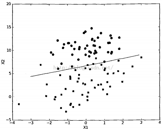
这里我们有100个样本点数据,每个数据有两个特征X1,X2;最后一列是标签分类
<span style="font-family:Microsoft YaHei;">from numpy import *def loadDataSet(): dataMat = []; labelMat = [] //首先定义两个数组,一个装数据一个装标签 fr = open('testSet.txt') //打开文件 for line in fr.readlines(): lineArr = line.strip().<strong>split()</strong> dataMat.append([1.0, float(lineArr[0]), float(lineArr[1])]) //X1,X2特征,前面加上X0=1 labelMat.append(int(lineArr[2])) return dataMat,labelMat //返回100*3 100 数组def sigmoid(inX): return 1.0/(1+exp(-inX)) //返回g(z) def<strong> gradAscent</strong>(dataMatIn, classLabels): //定义梯度上升的函数 dataMatrix = mat(dataMatIn) #convert to NumPy matrix转化为矩阵 labelMat = mat(classLabels).transpose() #convert to NumPy matrix<strong>转化为竖着的形式</strong> m,n = shape(dataMatrix) alpha = 0.001 maxCycles = 500 weights = ones((n,1)) //3行1列的全1矩阵 初始化权值全为1 for k in range(maxCycles): #heavy on matrix operations 500次迭代 h = sigmoid(dataMatrix*weights) //θX的计算 100*3 3*1 最后带入sigmoid error = (labelMat - h) //误差计算 即公式中的y-h 注意h是100*1的矩阵 weights = weights + alpha * <strong>dataMatrix.transpose()</strong>* error //使权值沿着error的方向更新迭代 注意data进行了转置 return weights //n个权值,θj</span>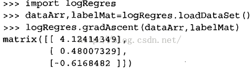
如何画出决策边界
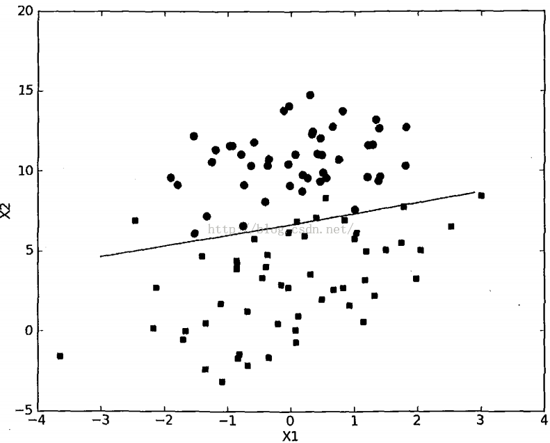
<span style="font-family:Microsoft YaHei;"> def plotBestFit(weights): import matplotlib.pyplot as plt dataMat,labelMat=loadDataSet() dataArr = array(dataMat) //转化为数组的形式 n = shape(dataArr)[0] //shape返回数组的大小,(100,3)的形式 n=100 xcord1 = []; ycord1 = [] //1类 xcord2 = []; ycord2 = [] //0类 for i in range(n): if int(labelMat[i])== 1: xcord1.append(dataArr[i,1]); ycord1.append(dataArr[i,2]) //如果属于1类 X1,Y1样本点坐标 else: xcord2.append(dataArr[i,1]); ycord2.append(dataArr[i,2]) //0类 x2,y2样本点坐标 fig = plt.figure() ax = fig.add_subplot(111) //把画布分成一行一列后在第一个位置画图 ax.scatter(xcord1, ycord1, s=30, c='red', marker='s') //画离散点 ax.scatter(xcord2, ycord2, s=30, c='green') x = arange(-3.0, 3.0, 0.1) //x坐标范围 y = (-weights[0]-weights[1]*x)/weights[2] //由0=W0X0+W1X1+W2X2得出X2的表达式,也就是纵坐标Y ax.plot(x, y) plt.xlabel('X1'); plt.ylabel('X2'); plt.show()</span>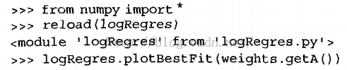
随机梯度上升算法:
我们发现这种批处理方法计算量往往比较大,每次都要计算所有的m个样本点同时还有所有的n个特征(或者说θ参数系数,特征的个数),所以我们引入随机梯度上升算法来简化计算量;随机梯度上升算法的特点是一次仅用一个样本点来更新回归系数;
def stocGradAscent0(dataMatrix, classLabels): m,n = shape(dataMatrix) alpha = 0.01 weights = ones(n) #初始化权值都为1,3*1 for i in range(m): //m个样本点 h = sigmoid(sum(<strong>dataMatrix[i]</strong>*weights)) //每次使用一个样本点来更新权值 error = <strong>classLabels[i]</strong> - h weights = weights + alpha * error * <strong>dataMatrix[i]</strong> return weights
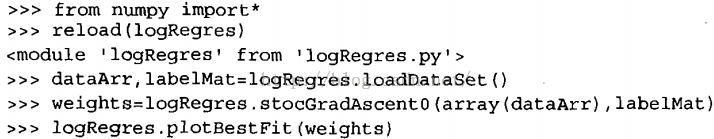
对比图我们发现此时的分界线并不完美,错误分类大约三分之一,我们将代码修改让其重复迭代200次后效果会更好;
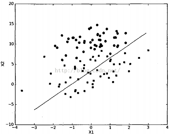
产生波动现象的原因是存在一些不能正确分类的样本点(数据集并非线性可分),在每次迭代时会引发系数的剧烈改变;
一种改进的随机梯度上升算法:
<span style="font-family:Microsoft YaHei;">def stocGradAscent1(dataMatrix, classLabels, numIter=150): m,n = shape(dataMatrix) weights = ones(n) #initialize to all ones for j in range(numIter): //150次迭代 dataIndex = range(m) for i in range<strong>(m)</strong>: //m次随机选取 alpha = 4/(1.0+j+i)+0.0001 </span>
<span style="font-family:Microsoft YaHei;"> #alpha每次迭代和每次的样本点都会调整,即调整步幅越来越小从而避免波动 但不会最后变为0,因为0.0001为了数据始终具有影响 randIndex = int(random.uniform(0,len(dataIndex))) #实际上alpha并非严格下降,比如j=1,i=200 j=2,i=100这个时候步幅是增大的 h = sigmoid(sum(dataMatrix<strong>[randIndex]</strong>*weights)) //通过随机选取避免周期性波动 error = classLabels<strong>[randIndex]</strong> - h weights = weights + alpha * error * dataMatrix<strong>[randIndex]</strong> del(dataIndex<strong>[randIndex]</strong>) //要删掉当前的index避免重复选到同一个样本点 return weights</span>
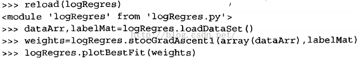
该方法比采用固定alpha的方法收敛速度更快,且分隔线达到了与Gradientascent()差不多的效果,但是所使用的计算量更少;
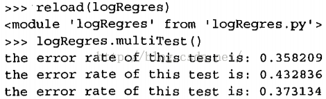
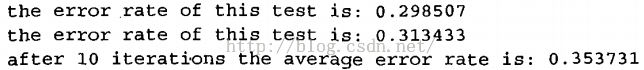
一个小例子:预测马的存活与否
数据是22列,即有21个特征,最后一列为样本标签;(一点数据清洗的问题,将缺失的特征置为0,缺失的标签舍去整个样本点)
<span style="font-family:Microsoft YaHei;">def classifyVector(inX, weights): prob = sigmoid(sum(inX*weights)) if prob > 0.5: return 1.0 else: return 0.0 //类别标签判断def colicTest(): frTrain = open('horseColicTraining.txt'); frTest = open('horseColicTest.txt') trainingSet = []; trainingLabels = [] for line in frTrain.readlines(): currLine = line.strip().split('\t') lineArr =[] for i in range(21): lineArr.append(float(currLine[i])) trainingSet.append(lineArr) trainingLabels.append(float(currLine[21])) trainWeights = stocGradAscent1(array(trainingSet), trainingLabels, 1000) //1000次迭代 errorCount = 0; numTestVec = 0.0 for line in frTest.readlines(): //测试模型 numTestVec += 1.0 //测试的样本点的个数 currLine = line.strip().split('\t') lineArr =[] for i in range(21): lineArr.append(float(currLine[i])) if int(classifyVector(array(lineArr), trainWeights))!= int(currLine[21]): //判断当前样本点是否与对应标签 errorCount += 1 errorRate = (float(errorCount)/numTestVec) print "the error rate of this test is: %f" % errorRate return errorRatedef multiTest(): numTests = 10; errorSum=0.0 for k in range(numTests): errorSum += colicTest() print "after %d iterations the average error rate is: %f" % (numTests, errorSum/float(numTests)) </span>运行结果: